
End-2-end Machine Learning Project with Python
Published:
The goal of this exercise is to go through the Machine Learning modeling process using Python.
I’ll recover the dataset I used in this and this blog posts about energy savings in building renovation strategies. Check them for further context.
The Machine Learning end-2-end project consists of the following steps:
- Selecting the performance measure
- Checking the modeling assumptions
- Quick exploration of data
- Creating the test set
- Exploring the data visually to gain insights
- Attribute combination A.K.A. Feature Engineering
- Preparing the data for ML models
- Model selection and training
- Analyzing errors to improve our model, and finally
- Model testing
Notice that the steps previous to the modeling phase are a lot, and indeed, those will take up most of our working time in a project like this.
I’ll drive you through each of the steps, going into enough detail to give you a general idea of how each works.
Performance measure
The performance measure is an indicator that gives an idea of how much error the system makes in its predictions. You’ll get an idea of what I’m talking about with this image.
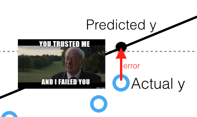
The performance measure for this project will be the Root Mean Squared Error (RMSE). It is a widely used error measure when it comes to Regression tasks[1]. It is described as follows:
\[RMSE(X,h)=\sqrt{\frac{1}{m}\sum^m_{i=1}(h(x^{(i)}) - y^{(i)})^2}\]Where,
- $X$ is the matrix containing all the features, excluding the label or target variable
- $h$ is the hypothesis, i.e., the model function
- $m$ is the length of the dataset, i.e., the number of instances or buildings in it
- $x^{(i)}$ is a vector of all the feature values (excluding the label) of the $i^{th}$ instance in the dataset. Hence, $h(x^{(i)})$ gives us the “predicted $y$”
- $y$ is the real target value
This performance measure imputes higher weight for large errors.
Asumptions
We have in our hands a regression task. We will use the data set to predict the building’s energy consumption.
The data I use for this post has some limitations. Mainly:
- the target variable is a calculated attribute,
- there will be errors and outliers derived from the data collection process
I assume that anyone that reaches this notebook will have some basic familiarity with Python and Machine Learning. Anyhow, I’ll try to do it as accessible as possible to someone with little to no knowledge.

Sometimes, variables are referred to as “attributes” or “features” while “attributes” is the preferred one.
Configuration
import numpy as np
import pandas as pd
import seaborn as sns
import geopandas as gpd
import shapefile as shp
import matplotlib as mpl
import matplotlib.pyplot as plt

from scipy import stats

%matplotlib inline
%config InlineBackend.figure_format ='retina'

mpl.rcParams['figure.figsize'] = (10, 6)
sns.set(style = 'whitegrid', font_scale = 1)
Get the data
buildings = pd.read_csv("../santboi/data/1906SB_collection_heatd.csv")
Quick Data Exploration
print('ORIGINAL DATA:')
buildings.info(null_counts=True)
ORIGINAL DATA:
<class 'pandas.core.frame.DataFrame'>
RangeIndex: 814 entries, 0 to 813
Data columns (total 20 columns):
 #   Column                     Non-Null Count  Dtype
---  ------                     --------------  -----
 0   X Coord                    746 non-null    float64
 1   Y Coord                    746 non-null    float64
 2   District                   814 non-null    object
 3   Year                       814 non-null    int64
 4   Main Orientation           814 non-null    object
 5   GF Usage                   814 non-null    object
 6   Roof Surface               814 non-null    float64
 7   Facade Surface             814 non-null    float64
 8   Openings Surface           814 non-null    float64
 9   Wrapping Surface           814 non-null    float64
 10  Party Wall Surface         814 non-null    float64
 11  Contact w/Terrain Surface  814 non-null    float64
 12  Type of Roof               814 non-null    object
 13  Type of Opening            814 non-null    object
 14  Type of Party Wall         814 non-null    object
 15  Type of Facade             814 non-null    object
 16  Number of Floors           814 non-null    int64
 17  Number of Courtyards       814 non-null    int64
 18  Number of Dwellings        814 non-null    int64
 19  Heat Demand                814 non-null    float64
dtypes: float64(9), int64(4), object(7)
memory usage: 127.3+ KB
Always print the data to see how it looks like.
buildings.head()
| X Coord | Y Coord | District | Year | Main Orientation | GF Usage | Roof Surface | Facade Surface | Openings Surface | Wrapping Surface | Party Wall Surface | Contact w/Terrain Surface | Type of Roof | Type of Opening | Type of Party Wall | Type of Facade | Number of Floors | Number of Courtyards | Number of Dwellings | Heat Demand | |
|---|---|---|---|---|---|---|---|---|---|---|---|---|---|---|---|---|---|---|---|---|
| 0 | 2.032087 | 41.348370 | Marianao | 1977 | E | Commercial | 165.43 | 208.50 | 56.1150 | 1473.28 | 150.9 | 150.00 | C2 | H4 | M2 | F3 | 5 | 1 | 5 | 44.251546 |
| 1 | 2.032074 | 41.348412 | Marianao | 1978 | W | Commercial | 417.41 | 547.35 | 218.9400 | 2524.31 | 36.6 | 420.00 | C2 | H3 | M2 | F3 | 5 | 2 | 19 | 38.328312 |
| 2 | 2.032024 | 41.348669 | Marianao | 1976 | E | Commercial | 202.00 | 282.00 | 112.8000 | 1637.97 | 108.9 | 202.07 | C2 | H3 | M2 | F3 | 5 | 2 | 14 | 58.794629 |
| 3 | 2.043332 | 41.338324 | Vinyets | 1959 | NW | Dwelling | 96.00 | 148.80 | 38.4024 | 489.60 | 0.0 | 96.00 | C1 | H3 | 0 | F1 | 3 | 0 | 2 | 126.321738 |
| 4 | 2.043382 | 41.338281 | Vinyets | 1958 | NE | Dwelling | 45.00 | 61.38 | 18.4170 | 418.31 | 0.0 | 80.00 | C1 | H4 | 0 | F1 | 2 | 1 | 2 | 69.562085 |
I got latitude and longitude via the Spanish Cadastre API. There are 68 nulls in those variables because some references have errors.
Let’s see how is our categorical data.
buildings["District"].value_counts()
Marianao    499
Vinyets     315
Name: District, dtype: int64
This is an important variable. As we know from the context study, the use case is highly dependent on the territory.
buildings["Main Orientation"].value_counts()
N     134
S     131
E     109
W     106
SE     98
NE     86
NW     79
SW     71
Name: Main Orientation, dtype: int64
buildings["GF Usage"].value_counts()
Dwelling      401
Commercial    355
Storage        41
Industrial     17
Name: GF Usage, dtype: int64
Let’s see some statistics of nuimerical data.
buildings.describe()
| X Coord | Y Coord | Year | Roof Surface | Facade Surface | Openings Surface | Wrapping Surface | Party Wall Surface | Contact w/Terrain Surface | Number of Floors | Number of Courtyards | Number of Dwellings | Heat Demand | |
|---|---|---|---|---|---|---|---|---|---|---|---|---|---|
| count | 746.000000 | 746.000000 | 814.000000 | 814.000000 | 814.000000 | 814.000000 | 814.000000 | 814.000000 | 814.000000 | 814.000000 | 814.000000 | 814.000000 | 814.000000 |
| mean | 2.037112 | 41.344455 | 1958.713759 | 188.012064 | 283.197881 | 92.051687 | 1174.339019 | 89.446564 | 191.163845 | 3.819410 | 1.067568 | 8.509828 | 78.686759 |
| std | 0.005807 | 0.004975 | 24.095145 | 162.277031 | 346.681371 | 154.381926 | 991.088501 | 144.038287 | 166.748749 | 1.811693 | 1.209477 | 10.797443 | 41.569118 |
| min | 2.028457 | 41.334829 | 1700.000000 | 30.080000 | 14.280000 | 2.570000 | 150.920000 | 0.000000 | 38.610000 | 1.000000 | 0.000000 | 1.000000 | 5.977362 |
| 25% | 2.032491 | 41.339325 | 1958.000000 | 91.000000 | 77.334300 | 18.899490 | 494.850000 | 0.000000 | 93.812500 | 2.000000 | 0.000000 | 1.000000 | 48.330863 |
| 50% | 2.034446 | 41.346671 | 1967.000000 | 129.565000 | 157.920000 | 40.266405 | 851.655000 | 33.985500 | 131.500000 | 4.000000 | 1.000000 | 4.000000 | 69.391495 |
| 75% | 2.043433 | 41.349227 | 1973.000000 | 224.587500 | 344.475000 | 94.001554 | 1497.847500 | 117.810000 | 225.532500 | 5.000000 | 2.000000 | 12.000000 | 99.243290 |
| max | 2.046343 | 41.352760 | 1979.000000 | 1367.000000 | 2765.940000 | 1795.254000 | 6159.730000 | 1287.270000 | 1405.000000 | 8.000000 | 7.000000 | 83.000000 | 233.075410 |
The only thing that catches my attention is that there is a high maximum for Heat Demand, far from its 3rd quantile.
Let’s complement them with plots.
buildings.hist(bins=50, figsize=(20,15))
plt.show()
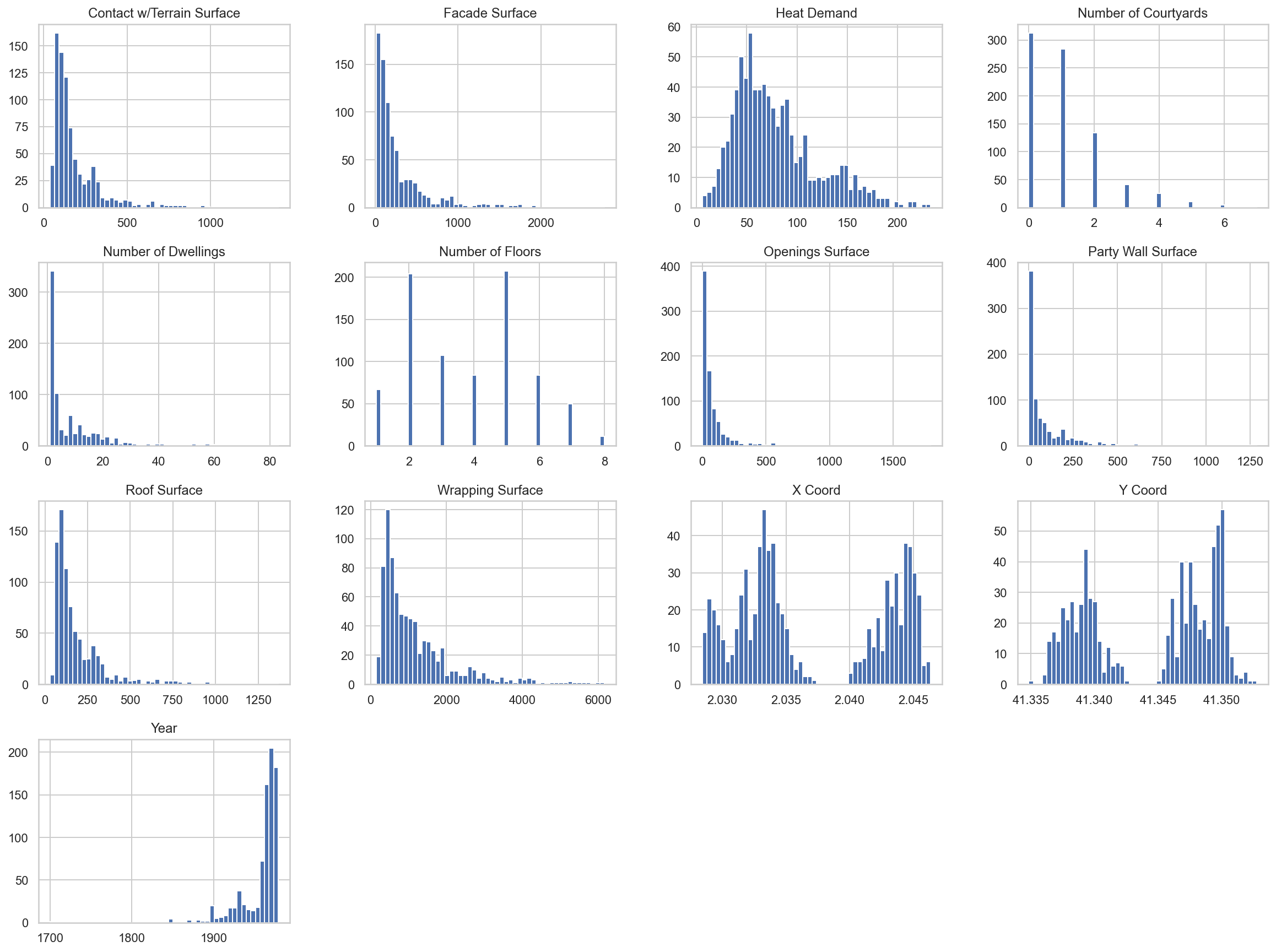
Now we can observe some peculiarities in data:
- Two numerical attributes,
Number of CourtyardsandNumber of floors, might be considered as categorical or numeric - Most buildings have 2 or 5 heights
- Many distributions are tail-heavy
- The Attributes have different scales
- Heat demand shows a bimodal distribution (i.e., two peaks). It indicates that an important category is producing this difference.
Create the Test Set
After getting a quick look at the data, the next thing we need to do is putting aside the test set (i.e., the dataset we will use to test our model’s performance with data that it does not know) to ignore it until the appropriate moment.
The approach of this study is territory-wise. It must be taken into account when splitting the dataset in the train and test set. Data in both sets must be representative of each District.
Another fundamental attribute is Number of Floors. Hence, data is stratified concerning this variable too.
Here, the proportions in the whole dataset for both variables.
print("DISTRICT PROPORTIONS:")
buildings["District"].value_counts(normalize=True)
DISTRICT PROPORTIONS:
Marianao    0.613022
Vinyets     0.386978
Name: District, dtype: float64
print("NUMBER OF FLOORS PROPORTIONS:")
buildings["Number of Floors"].value_counts(normalize=True)
NUMBER OF FLOORS PROPORTIONS:
5    0.254300
2    0.250614
3    0.131450
6    0.103194
4    0.103194
1    0.082310
7    0.061425
8    0.013514
Name: Number of Floors, dtype: float64
Now we are prepared to implement Scikit-Learn’s StratifiedShuffleSplit class. You will see that Scikit-Learn classes are used in several moments. This is the best practice when it comes to automate and make reproducible all the steps in a Machine Learning Project conducted with python.
from sklearn.model_selection import StratifiedShuffleSplit

split = StratifiedShuffleSplit(n_splits=1, test_size=0.2, random_state=42)
for train_index, test_index in split.split(buildings, buildings.loc[:,("District", "Number of Floors")]):
    buildings_train_set = buildings.loc[train_index]
    buildings_test_set = buildings.loc[test_index]
print("DISTRICT PROPORTIONS IN TEST SET:")
buildings_test_set["District"].value_counts(normalize=True)
DISTRICT PROPORTIONS IN TEST SET:
Marianao    0.613497
Vinyets     0.386503
Name: District, dtype: float64
print("NUMBER OF FLOORS PROPORTIONS IN TEST SET:")
buildings_test_set["Number of Floors"].value_counts(normalize=True)
NUMBER OF FLOORS PROPORTIONS IN TEST SET:
5    0.257669
2    0.251534
3    0.128834
6    0.104294
4    0.104294
1    0.085890
7    0.055215
8    0.012270
Name: Number of Floors, dtype: float64
Exploring Data Visually to Gain Insights
Univariate analysis was already performed. Clic here to see more.
This exploration is performed over the training data to avoid early catching patterns in the test data.
buildings = buildings_train_set.copy()
import matplotlib.patches as patches

x = buildings["X Coord"]
y = buildings["Y Coord"]
s = buildings["Number of Dwellings"]
hd = buildings["Heat Demand"]
label = buildings["Number of Dwellings"]
cmap=plt.get_cmap('jet')

sb_map = plt.imread("/images/blog/end-2-end-ml-python/map.png")
bbox = (2.024, 2.049, 41.334, 41.355)

fig = plt.figure(figsize=(4*7,3*7))
ax = plt.subplot(221)
scat = plt.scatter(x=x, y=y, label=label, alpha=0.4, s=s*10, c=hd, cmap=cmap)
ax.set_xlim(bbox[0],bbox[1])
ax.set_ylim(bbox[2],bbox[3])
plt.imshow(sb_map, zorder=0, extent = bbox, aspect='equal')
plt.colorbar(scat, label="Heat Demand")
ax.legend(["Number of Dwellings"])

plt.show()
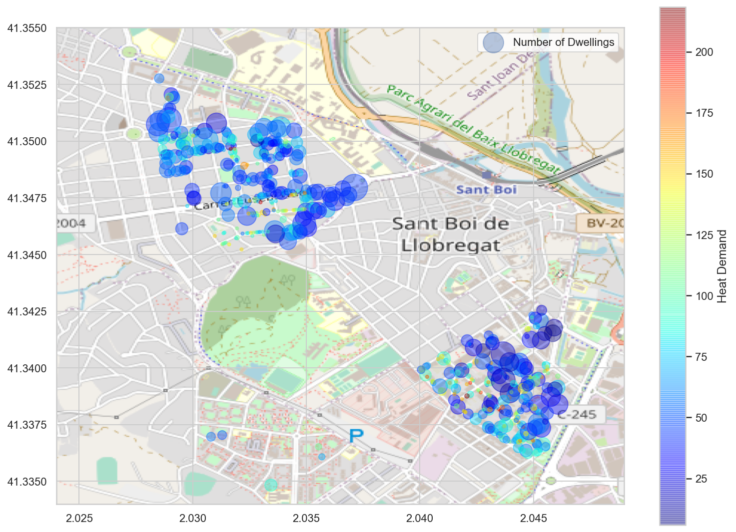
Credits to openstreemap.org for the image in the background.
Some things we can notice examining the map are:
- The small buildings, represented with small circles, tend to be red or clear blue. It means that their estimated Heat Demand is higher.
- The size of the building is undoubtedly a determining attribute when it comes to heat demand.
Correlations
To measure the correlation between variables, we can calculate the Pearson’s correlation coefficient. This will give us an idea of the linear correlations between variables. In our case, we want to see how all variables correlate with our target variable, which is Heat Demand.
To interpret it, we should know that:
- Strong correlations exist as the Pearson’s correlation coefficient comes close to
1or-1. They are considered to be negatively strong when lower than-0.5and positively strong when higher than0.5. - When it is positive, it means that there is a positive correlation, or that both compared variables increase in the same direction. When it is negative, as one of the compared variables increases, the other does the opposite.
- Values closer to 0 are indicating weaker linear correlations.
corr_matrix = buildings.corr()
corr_matrix["Heat Demand"].sort_values(ascending=False)
Heat Demand                  1.000000
X Coord                      0.138257
Party Wall Surface          -0.116543
Y Coord                     -0.217586
Number of Courtyards        -0.264093
Roof Surface                -0.341468
Contact w/Terrain Surface   -0.375108
Openings Surface            -0.403764
Facade Surface              -0.420780
Year                        -0.439196
Number of Dwellings         -0.458880
Wrapping Surface            -0.464788
Number of Floors            -0.635959
Name: Heat Demand, dtype: float64
We can complement this matrix with a heat map, representing the above calculations in a more intuitive way.
plt.figure(figsize = (8,8))
corr = buildings.corr()
cmap = sns.diverging_palette(220, 10, as_cmap=True)
sns.heatmap(
    corr, cmap=cmap, square=True, cbar=False,
    annot=True, annot_kws={'fontsize':12}
)
plt.yticks(rotation=0)
plt.xticks(rotation=90)
plt.show()
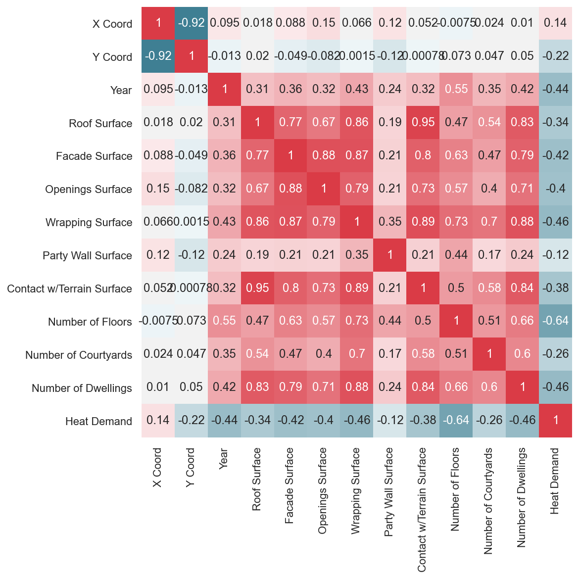
As you can see at the heat map, the correlations with the response attribute Heat Demand are not specially marked. However, many of the explanatory variables are strongly correlated with each other.
See, for example, Contact w/Terrain Surface and Roof Surface. If we think about a perfectly cubic building, each of these two measurements will be the same. In reality, many buildings have varying shapes from their base to the roof, so they are not perfectly correlated. However, the linear correlation is pretty high anyway.
This phenomenon of high correlations between predictor attributes is known as multicolinearity, and it’s something that we do not want for our models. They are attributes that are considered redundant, so it is unnecessary to have both in the model. Otherwise, you’d only be adding noise to the system.
Tree-based algorithms handle this phenomenon well, while other models might be more sensitive to it. We could try what happens if we consider all of them or if we take the one with the highest correlation coefficient (i.e., Wrapping Surface).
We can get a better idea of how variables correlate with scatter plots. In the following, you can see how some patterns appear in the scatterplots (focus on the first row).
In the diagonal, you will find the histogram corresponding to the variable on the y axis.
As there is only one instance from the year 1700, it is removed from the plots to get a better idea of the patterns.
from pandas.plotting import scatter_matrix

exclude = ["X Coord", "Y Coord", "Number of Floors", "Number of Courtyards", "Number of Dwellings"]
sm = scatter_matrix(buildings.loc[buildings.Year > 1800, [c for c in buildings.columns if c not in exclude]], figsize=(16,9))
for subaxis in sm:
    for ax in subaxis:
        l = ax.get_ylabel()
        ax.set_ylabel(l, rotation=0, ha="right")

plt.show()
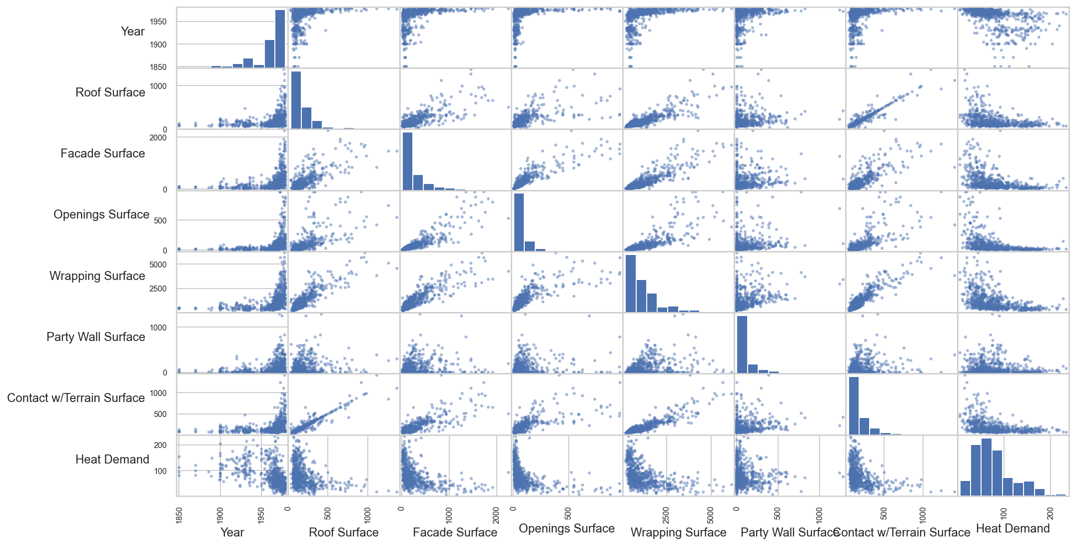
- All the surface attributes have a very similar relationship with
Heat Demand. - Most of the buildings were built from 1960 and on (the two last higher bars).
- There seem to be logarithmic correlations between most attributes and
Heat Demand.
Attribute Combination A.K.A. Feature Engineering
Feature Engineering is the step that usually makes the difference in an ML project. Knowing the subject and its complexity can help you produce new attributes that can improve the models enormously.
To keep it simple, I’ll only try a simple logarithmic transformation on the surface variables. But the best you can do is try all the combinations that you can get. We’ll leave Party Wall Surface out, as it has many zero values and this will break our workflow.
surface_attrs = [col for col in buildings.columns if "Surface" in col]
surface_attrs = [a for a in surface_attrs if a != "Party Wall Surface"]

for attr in surface_attrs:
    buildings["Log "+attr] = np.log(buildings[attr].replace(0, np.nan))
And now let’s compute the correlations again.
corr_matrix = buildings.corr()
corr_matrix["Heat Demand"].sort_values(ascending=False)
Heat Demand                      1.000000
X Coord                          0.138257
Party Wall Surface              -0.116543
Y Coord                         -0.217586
Number of Courtyards            -0.264093
Roof Surface                    -0.341468
Log Roof Surface                -0.364450
Contact w/Terrain Surface       -0.375108
Openings Surface                -0.403764
Log Contact w/Terrain Surface   -0.414675
Facade Surface                  -0.420780
Year                            -0.439196
Number of Dwellings             -0.458880
Wrapping Surface                -0.464788
Log Facade Surface              -0.543432
Log Wrapping Surface            -0.555474
Log Openings Surface            -0.587757
Number of Floors                -0.635959
Name: Heat Demand, dtype: float64
Not surprisingly, all the transformed attributes got a stronger (negative) linear correlation with Heat Demand. Here is how these transformed variables look like when plotted against our target variable.
x1 = np.array(buildings["Wrapping Surface"])
x2 = np.array(buildings["Log Wrapping Surface"])
y = np.array(buildings["Heat Demand"])

m1, b1 = np.polyfit(x1, y, 1)
m2, b2 = np.polyfit(x2, y, 1)

fig, ax = plt.subplots(1,2)

ax[0].scatter(x1, y, alpha = .5, c="grey")
ax[0].plot(x1, m1*x1 + b1, c="grey")

ax[0].set_xlabel("Wrapping Surface", fontsize=15)
ax[0].set_ylabel("Heat Demand", fontsize=15)
ax[0].set_title("Relationship before the transformation")

ax[1].scatter(x2, y, alpha = .5)
ax[1].plot(x2, m2*x2 + b2)

ax[1].set_xlabel("Log of Wrapping Surface", fontsize=15)
ax[1].set_ylabel("Heat Demand", fontsize=15)
ax[1].set_title("Relationship after the transformation")

plt.show()
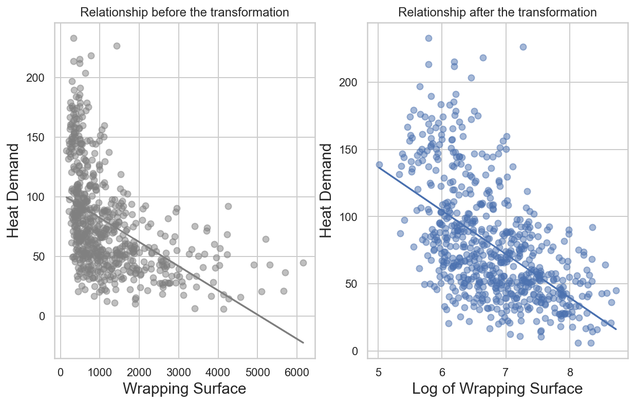
Definitely better!
Prepare Data for ML ALgorithms
The first thing is to revert to a clean training set and separate predictors from labels, as we don’t necessarily want to apply the same transformations to each one of them.
We’ll work with a copy of buildings_train_set, overwriting buildings as we did earlier (notice that drop() will create a copy of the data and it does not affect buildings_train_set).
buildings = buildings_train_set.drop("Heat Demand", axis=1)
buildings_labels = buildings_train_set["Heat Demand"].copy()
Outliers
Data preparation must include outlier removal. Outliers, or in other words, data noise, produce less consistent models. Let’s plot the distribution of the target variable to see if we can easily detect outliers.
sns.boxplot(x=buildings_labels)
plt.show()
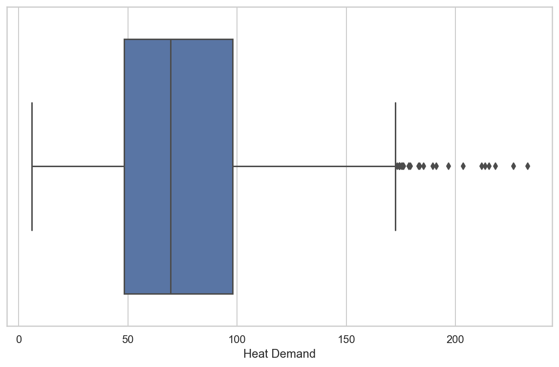
As we can see above, there are a few points over the 75% quantile of the distribution (to the right of the boxplot’s rightest whisker). It is hard to determine if all of them should be considered outliers.
It seems that there isn’t a clear boundary between the points that are outliers and those that aren’t. So, instead of using the IQR method (i.e., delete outliers based on the boxplot), let’s use the z-score method. It is suitable as Heat Demand shows a distribution similar to the normal.
from scipy import stats
import numpy as np

def drop_outliers_by_zscore(s, threshold=3):
    z_score = np.abs(stats.zscore(s))
    idx = np.where(z_score < threshold)
    return s.iloc[idx[0],]
buildings_labels_z = drop_outliers_by_zscore(buildings_labels, threshold=3)
sentence = "Instances deleted: "
pctg = 100*(buildings_labels.shape[0] - buildings_labels_z.shape[0]) / (buildings_labels.shape[0])
print(sentence, "{:.2f}% of the data".format(pctg))
Instances deleted: 0.92% of the data
Finally, we can overwrite the buildings variable without the outliers.
buildings = buildings.loc[buildings_labels_z.index]
buildings_labels = buildings_labels.loc[buildings_labels_z.index]
Categorical Attributes
The following are the categorical attributes in the dataset.
buildings_cat = buildings.select_dtypes(("object", "category"))
buildings_cat_names = buildings_cat.columns.values.tolist()
buildings_cat_names
['District',
 'Main Orientation',
 'GF Usage',
 'Type of Roof',
 'Type of Opening',
 'Type of Party Wall',
 'Type of Facade']
Machine Learning Models require numerical data to be able to work. Then, we should treat categorical data before feeding ML models with them.
As we won’t consider an order relationship between categories, we will replace the categorical attributes with dummy variables. It means replacing the categorical attribute with a new column for each category in it and then assigning a 1 for the column corresponding to the instance’s category and a 0 for the rest.
from sklearn.preprocessing import OneHotEncoder

cat_encoder = OneHotEncoder()
buildings_cat_1hot = cat_encoder.fit_transform(buildings_cat)
Now, each column in the array corresponds to a category in the original attribute.
Custom Transformers
Custom Transformers will allow us to produce more complex data preparation steps than the standard ones provided by Scikit-Learn.
We need to create a custom class to transform our surface variables to their logarithm.
from sklearn.base import BaseEstimator, TransformerMixin

roof_idx, facade_idx, openings_idx = 3, 4, 5
wrapping_idx, party_idx, terrain_idx = 6, 7, 8

class LogTransformAttrs(BaseEstimator, TransformerMixin):
    def __init__(self, log_transform_attrs=True):
        self.log_transform_attrs = log_transform_attrs
    def fit(self, X, y=None):
        return self
    def transform(self, X):
        if not self.log_transform_attrs:
            return X
        else:
            X = np.array(X)
            X[:,roof_idx] = np.log(X[:,roof_idx])
            X[:,facade_idx] = np.log(X[:,facade_idx])
            X[:,openings_idx] = np.log(X[:,openings_idx])
            X[:,wrapping_idx] = np.log(X[:,wrapping_idx])
            X[:,terrain_idx] = np.log(X[:,terrain_idx])
            return X
Feature Scaling
The year a building was built has a very different scale than the number of floors it can have. This can degrade the predictive performance of many machine learning algorithms.
To tackle this, we can use scaling techniques. Here, we will try several methods to go beyond the default class used in many Machine Learning Projects StandardScaler(). Scikit-Learn provides several classes to do so.
We will test no scaling too.
from sklearn.preprocessing import MinMaxScaler, StandardScaler, MaxAbsScaler, RobustScaler

class CustomScaler(BaseEstimator, TransformerMixin):
    """
    Choose one of the following values for the scaler parameter:
    -  None: Data wont be scaled
    - 'standard': StandardScaler()
    - 'minmax': MinMaxScaler()
    - 'maxabs': MaxAbsScaler()
    - 'robust': RobustScaler()
    """
    def __init__(self, scaler='standard'):
        valid_scalers = [None, 'standard', 'minmax', 'maxabs', 'robust']
        self.scaler = scaler
    def fit(self, X, y=None):
        return self
    def transform(self, X):
        if self.scaler is None:
            return np.array(X)
        elif self.scaler == 'standard':
            return StandardScaler().fit_transform(X)
        elif self.scaler == 'minmax':
            return MinMaxScaler().fit_transform(X)
        elif self.scaler == 'maxabs':
            return MaxAbsScaler().fit_transform(X)
        elif self.scaler == 'robust':
            return RobustScaler().fit_transform(X)
        else:
            raise ValueError("Invalid Scaler: '{}'; choose one of:\n {}".format(self.scaler, valid_scalers))
For more information on how these classes work, visit this page.
Transformation Pipelines
To have better control over the transformation process, we implement Pipelines. It prevents us from doing each step manually. With Pipelines, every stage of the transformation process is produced automatically in the stipulated order. The output of the preceding stage will be the input of the following one.
Together with the custom transformers, Pipelines will make these transformations optional and combinable in an automated manner. Thus we can test which mix of hyperparameters gives us the best model performance.
Most algorithms are not able to deal with missing values. Let’s use a transformation to deal with them and include this transformation in a pipeline.
Here, we will try the Scikit-Learn’s KNNImputer. This imputer will take the mean of its k nearest neighbors. The nearest neighbors are selected through the euclidean distance between individuals, taking into account all attributes.
Let’s create a pipeline to deal with the numerical attributes.
from sklearn.pipeline import Pipeline
from sklearn.impute import KNNImputer

num_pipeline = Pipeline([
    ('knn_imputer', KNNImputer(n_neighbors=3, weights="uniform")),
    ('log_transform_attrs', LogTransformAttrs(log_transform_attrs=True)),
    ('custom_scaler', CustomScaler(scaler='standard'))
])
Next, we should include a pipeline to transform categorical attributes, to make our models able to deal with them.
With the categorical pipeline, we will impute one-hot encoding over all the categorical attributes to transform them into dummy variables.
cat_pipeline = Pipeline([
    ('one_hot_encoder', OneHotEncoder())
])
Finally, we use the ColumnTransformer() class to implement all transformations (over numerical and categorical data) in the same pipeline.
from sklearn.compose import ColumnTransformer

buildings_num = buildings.select_dtypes(("float64", "int64"))

num_attribs = list(buildings_num.columns.values)
cat_attribs = list(buildings_cat.columns.values)

full_pipeline = ColumnTransformer([
    ("num", num_pipeline, num_attribs),
    ("cat", cat_pipeline, cat_attribs)
])

buildings_prepared = full_pipeline.fit_transform(buildings)
Model Selection and Training
The hardest work is already done! We have gone through data exploration, visual analysis, and the data preparation steps. Those usually are the most time-consuming ones. The following steps are where the fun part is. Let’s dive into the models!
This step consists of trying out several models (those suited for a regression task, in this case) to see which performs best. Let’s start simply by training a Linear Regression first.
from sklearn.linear_model import LinearRegression

lin_reg = LinearRegression()
lin_reg.fit(buildings_prepared, buildings_labels)
LinearRegression()
Let’s print some target values and some predictions to see how it is working.
some_data = buildings.iloc[:5]
some_labels = buildings_labels.iloc[:5]
some_data_prepared = full_pipeline.transform(some_data)
print("Predictions:", lin_reg.predict(some_data_prepared))
Predictions: [110.47113194 114.3593365 69.76232371 69.71247099 35.47188548]
print("Labels:", list(some_labels))
Labels: [83.80830072, 88.95706649, 53.80141858, 88.2675733, 12.44289642]
It works, although the predictions are not exactly accurate. Let’s measure this Regression Model’s RMSE on the whole training set. We are using Scikit-Learn’s mean_squared_error() function to do this.
from sklearn.metrics import mean_squared_error

buildings_predictions = lin_reg.predict(buildings_prepared)
lin_mse = mean_squared_error(buildings_labels, buildings_predictions)
lin_rmse = np.sqrt(lin_mse)
lin_rmse
24.00503744923763
It is not a bad score at all. Heat Demand ranges from 6 to over 200 kWh, so a typical prediction error of 23.6 kWh is not a big deal.
from sklearn.tree import DecisionTreeRegressor

tree_reg = DecisionTreeRegressor()
tree_reg.fit(buildings_prepared, buildings_labels)
DecisionTreeRegressor()
buildings_predictions = tree_reg.predict(buildings_prepared)
tree_mse = mean_squared_error(buildings_labels, buildings_predictions)
tree_rmse = np.sqrt(tree_mse)
tree_rmse
0.0
It could seem like we have found the perfect model, but slow down! It is more likely that the model is overfitting than it is perfect.
At this point, it is important to remember that we don’t want to touch the test set until we are ready to launch a model that we are confident about, so before doing this, we will use a part of the training set and part of it for validation in operation known as cross-validation.
Using Cross-Validation to Evaluate Models
In short, cross-validation is an iterative process that consists of training the model in different subsets of the (training) data to then get the final predictions by averaging each step’s results iteration. We use the technique to be sure that the outcome is independent of the partition of the data.
The fastest way to implement cross-evaluation is using the Scikit-Learn’s K-fold cross validation feature. The following code randomly splits the training set into ten distinct subsets called folds, then trains and evaluates the Decision Tree model 10 times, picking a different fold for evaluation every time and training on the other nine folds. The result is an array containing the ten evaluation scores.
from sklearn.model_selection import cross_val_score
scores = cross_val_score(tree_reg, buildings_prepared, buildings_labels,
                        scoring="neg_mean_squared_error", cv=10)
tree_rmse_scores = np.sqrt(-scores)
This process will output a series of 10 scores, one for each cross validation set. We can average errors to get the overall score.
def display_result(scores):
    print("Scores: ", scores)
    print("Mean: ", scores.mean())
    print("Std Deviation: ", scores.std())

display_result(tree_rmse_scores)
Scores:  [31.13854729 27.57049085 37.70195471 37.59302751 40.43146213 31.10880935
 29.56610138 33.69169129 33.71245778 34.55008854]
Mean:  33.70646308335529
Std Deviation:  3.8097460977538105
A RandomForestRegressor, is an esamble method. It takes several trees and averages the results of their predictions.
from sklearn.ensemble import RandomForestRegressor

forest_reg = RandomForestRegressor(random_state=42)
forest_reg.fit(buildings_prepared, buildings_labels)
RandomForestRegressor(random_state=42)
%%time
scores = cross_val_score(forest_reg, buildings_prepared, buildings_labels,
                         scoring="neg_mean_squared_error", cv=10)
forest_rmse_scores = np.sqrt(-scores)
CPU times: user 5.53 s, sys: 118 ms, total: 5.65 s
Wall time: 6.15 s
Aknowledge that we have to compute the -scores because Scikit-Learn’s cross-validation feature expects a utility function (greater is better) rather than a cost function (lower is better), so the scoring is actually the opposite of the MSE
buildings_predictions = forest_reg.predict(buildings_prepared)
forest_mse = mean_squared_error(buildings_labels, buildings_predictions)
forest_rmse = np.sqrt(forest_mse)
forest_rmse
8.411223538977632
display_result(forest_rmse_scores)
Scores:  [19.12399547 23.28758396 23.37826397 22.66663702 26.36400628 21.86384703
 23.60862608 21.41029322 24.67920191 25.51854666]
Mean:  23.190100162245255
Std Deviation:  1.9916505969479534
Random Forests seems to work better than Linear Regression! However, notice that the train set score is relatively lower than in the validation sets. It is due to overfitting in the training set. The possible solutions to this common Machine Learning problem are:
- Getting more data
- Feeding the model with new and more significant attributes
- Regularizing the model, i.e., use hyperparameters to apply constraints over it.
We have to try several other models before diving deeper into the next step (fine-tuning). E.g., we could try out Support Vector Machines with different kernels, and possibly a neural network, without spending too much time tweaking the hyperparameters. The goal is to shortlist a few (two to five) promising models.
Let’s, then, try the Scikit-Learn’s Super Vector Machine Regressor (SVR).
from sklearn.svm import SVR

svm_reg_linear = SVR(kernel='linear')
svm_reg_linear.fit(buildings_prepared, buildings_labels)
svm_linear_scores = cross_val_score(svm_reg_linear, buildings_prepared, buildings_labels,
                             scoring="neg_mean_squared_error", cv=10)
svm_linear_rmse_scores = np.sqrt(-scores)
svm_linear_rmse_scores.mean()
23.190100162245255
buildings_predictions = svm_reg_linear.predict(buildings_prepared)
svm_linear_mse = mean_squared_error(buildings_labels, buildings_predictions)
svm_linear_rmse = np.sqrt(svm_linear_mse)
svm_linear_rmse
25.140051958709613
And now with a rbf kernel.
svm_reg_rbf = SVR(kernel='rbf')
svm_reg_rbf.fit(buildings_prepared, buildings_labels)
svm_rbf_scores = cross_val_score(svm_reg_rbf, buildings_prepared, buildings_labels,
                             scoring="neg_mean_squared_error", cv=10)
svm_rbf_rmse_scores = np.sqrt(-scores)
svm_rbf_rmse_scores.mean()
23.190100162245255
buildings_predictions = svm_reg_rbf.predict(buildings_prepared)
svm_rbf_mse = mean_squared_error(buildings_labels, buildings_predictions)
svm_rbf_rmse = np.sqrt(svm_rbf_mse)
svm_rbf_rmse
31.13253629902029
The SVR’s RMSE is a little bit worse than the RandomForestRegressor’s one.
Since there is not much difference in the point estimates of the generalization error between the models we tried out, we may not be sure to decide on one of them.
To get a better idea of how our models perform and decide on one of them, we can set a 95% confidence interval for the generalization error using scipy.stats.t.interval().
predictions = {
    "lin_reg": lin_reg.predict(buildings_prepared),
    "forest_reg": forest_reg.predict(buildings_prepared),
    "svm_linear": svm_reg_linear.predict(buildings_prepared),
    "svm_rbf": svm_reg_rbf.predict(buildings_prepared)
}
from scipy import stats

confidence = .95

for key in predictions.keys():
    print(key)
    squared_errors = []
    for i in range(len(buildings_labels)):
        squared_errors.append((predictions[key][i] - buildings_labels.iloc[i]) ** 2)
    if key == "forest_reg":
        intervals = [forest_rmse_scores.mean()-forest_rmse_scores.std(), forest_rmse_scores.mean()+forest_rmse_scores.std()]
    else:
        squared_errors = np.array(squared_errors)
        intervals = np.sqrt(stats.t.interval(confidence, len(squared_errors) - 1, # minus one degree of freedom
                                                loc=np.mean(squared_errors),
                                                scale=stats.sem(squared_errors)))
    print(intervals)
lin_reg
[22.41800924 25.4934601 ]
forest_reg
[21.198449565297302, 25.181750759193207]
svm_linear
[23.22185601 26.92192096]
svm_rbf
[28.93537335 33.18454161]
At this point, we could choose almost any model that we have tried. See how all intervals overlap with each other? The obtained scores are not that different. In this type of scenario, we should opt for explainability (it’s convenient to know what models are doing).
From the models tried, Linear Regression and Random Forest are the most explainable ones.
Random Forest is slightly better than Linear Regression. We will choose the first one to go through the final steps: fine-tuning and testing the model.
Fine-Tunning
Now that we have selected our model, it is time to try out several parameters to make it the best possible. A common approach is using Scikit-Learn’s GridSearch(). We provide a series of parameters, and the algorithm will try all the possible combinations to search for the one which leads to the best result.
The main problem with this approach is that we generally do not know estimate an adequate range for an optimal parameter.
Instead, we can assess another approach to look for the best parameters for a model, the Scikit-Learn’s RandomizedSearchCV() class. The latter usually means achieving better results in the same amount of time.
In this case, we can stipulate any random distribution to search for each parameter. As our parameters are integers, we will use the scipy.stats.randint() function that generates a discrete uniform distribution in which any value in the range provided is equally likely to happen.
%%time
from sklearn.model_selection import RandomizedSearchCV
from scipy.stats import randint

param_distrib = {
    'bootstrap': [True, False],
    'n_estimators':randint(1,1000),
    'max_features': randint(4,35)
}

forest_reg = RandomForestRegressor()
random_search = RandomizedSearchCV(forest_reg, param_distrib, n_iter=50,
                                   cv=5, n_jobs=2, random_state=42,
                                   scoring='neg_mean_squared_error')
random_search.fit(buildings_prepared, buildings_labels)
CPU times: user 3.1 s, sys: 173 ms, total: 3.27 s
Wall time: 4min 28s

RandomizedSearchCV(cv=5, estimator=RandomForestRegressor(), n_iter=50, n_jobs=2,
                   param_distributions={'bootstrap': [True, False],
                                        'max_features': <scipy.stats._distn_infrastructure.rv_frozen object at 0x7f803dd21d00>,
                                        'n_estimators': <scipy.stats._distn_infrastructure.rv_frozen object at 0x7f803dd1b3a0>},
                   random_state=42, scoring='neg_mean_squared_error')
negative_mse = random_search.best_score_
rmse = np.sqrt(-negative_mse)
rmse
23.41819475588318
The best parameters for the model were the following.
random_search.best_params_
{'bootstrap': True, 'max_features': 24, 'n_estimators': 615}
Now that it is all set, it is time to implement a single pipeline with preparation and prediction.
from sklearn.model_selection import RandomizedSearchCV

prepare_select_and_predict_pipeline = Pipeline([
    ('preparation', full_pipeline),
    ('forest_prediction', RandomForestRegressor(**random_search.best_params_))
])

prepare_select_and_predict_pipeline.fit(buildings, buildings_labels)
Pipeline(steps=[('preparation',
                 ColumnTransformer(transformers=[('num',
                                                  Pipeline(steps=[('knn_imputer',
                                                                   KNNImputer(n_neighbors=3)),
                                                                  ('log_transform_attrs',
                                                                   LogTransformAttrs()),
                                                                  ('custom_scaler',
                                                                   CustomScaler())]),
                                                  ['X Coord', 'Y Coord', 'Year',
                                                   'Roof Surface',
                                                   'Facade Surface',
                                                   'Openings Surface',
                                                   'Wrapping Surface',
                                                   'Party Wall Surface',
                                                   'Contact w/Terrain Surface',
                                                   'Number of Floors',
                                                   'Number of Courtyards',
                                                   'Number of Dwellings']),
                                                 ('cat',
                                                  Pipeline(steps=[('one_hot_encoder',
                                                                   OneHotEncoder())]),
                                                  ['District',
                                                   'Main Orientation',
                                                   'GF Usage', 'Type of Roof',
                                                   'Type of Opening',
                                                   'Type of Party Wall',
                                                   'Type of Facade'])])),
                ('forest_prediction',
                 RandomForestRegressor(max_features=24, n_estimators=615))])
Let’s see how does the predictions look like.
some_data = buildings[:4]
some_labels = buildings_labels[:4]

print("Predictions:\t", prepare_select_and_predict_pipeline.predict(some_data))
print("Labels:\t\t", list(some_labels))
Predictions:	 [114.22055767 103.5844614   47.41711586  81.08963433]
Labels:		 [83.80830072, 88.95706649, 53.80141858, 88.2675733]
Looks great! Do you think that we can improve these predictions a bit more? We have tried out a grid search for the model’s parameters. But, what about the parameters of the data preparation step? Let’s explore them! This time I’ll use the GridSearch() class.
# uncomment to see pipeline avilable parameters
# prepare_select_and_predict_pipeline.get_params().keys()
%%time
from sklearn.model_selection import GridSearchCV

param_grid = [{
    'preparation__num__knn_imputer__n_neighbors': range(2,5),
    'preparation__num__log_transform_attrs__log_transform_attrs': [True, False],
    'preparation__num__custom_scaler__scaler': [None, 'standard', 'minmax', 'robust']
}]

grid_search_prep = GridSearchCV(prepare_select_and_predict_pipeline, param_grid=param_grid,
                                cv=5, scoring='neg_mean_squared_error')

grid_search_prep.fit(buildings, buildings_labels)
CPU times: user 5min 1s, sys: 5.87 s, total: 5min 7s
Wall time: 4min 31s

GridSearchCV(cv=5,
             estimator=Pipeline(steps=[('preparation',
                                        ColumnTransformer(transformers=[('num',
                                                                         Pipeline(steps=[('knn_imputer',
                                                                                          KNNImputer(n_neighbors=3)),
                                                                                         ('log_transform_attrs',
                                                                                          LogTransformAttrs()),
                                                                                         ('custom_scaler',
                                                                                          CustomScaler())]),
                                                                         ['X '
                                                                          'Coord',
                                                                          'Y '
                                                                          'Coord',
                                                                          'Year',
                                                                          'Roof '
                                                                          'Surface',
                                                                          'Facade '
                                                                          'Surface',
                                                                          'Openings '
                                                                          'Surface',
                                                                          'Wrapping '
                                                                          'Surface',
                                                                          'Party '
                                                                          'Wal...
                                                                          'Facade'])])),
                                       ('forest_prediction',
                                        RandomForestRegressor(max_features=24,
                                                              n_estimators=615))]),
             param_grid=[{'preparation__num__custom_scaler__scaler': [None,
                                                                      'standard',
                                                                      'minmax',
                                                                      'robust'],
                          'preparation__num__knn_imputer__n_neighbors': range(2, 5),
                          'preparation__num__log_transform_attrs__log_transform_attrs': [True,
                                                                                         False]}],
             scoring='neg_mean_squared_error')
We can access the best_params_ attribute inside our grid_search_prep object.
grid_search_prep.best_params_
{'preparation__num__custom_scaler__scaler': None,
 'preparation__num__knn_imputer__n_neighbors': 4,
 'preparation__num__log_transform_attrs__log_transform_attrs': False}
It’s expected for a Random Forest. They handle well different scales and non-linear predictor variables.
Saving models
As you may have notice, training a model or fine-tuning could be a very time-consuming process. Instead of doing it repeatedly, we can save our results with the joblib library.
import joblib

joblib.dump(grid_search_prep, "models/grid_search_prep.pkl")
['models/grid_search_prep.pkl']
And then, we can load it again with the following code:
grid_search_prep = joblib.load("models/grid_search_prep.pkl")
Analyzing Errors
We might be interested in gaining insight into what is happening with the best model. To do that, we can start by looking at each feature’s relative importance in the Random Forest model.
feature_importances = random_search.best_estimator_.feature_importances_

cat_encoder = full_pipeline.named_transformers_["cat"]["one_hot_encoder"]
cat_one_hot_attribs = cat_encoder.get_feature_names(cat_attribs)

attributes = num_attribs + list(cat_one_hot_attribs)

sorted(zip(feature_importances, attributes), reverse=True)
[(0.21736613066989782, 'Number of Floors'),
 (0.18726931676902742, 'Type of Roof_C2'),
 (0.09612240406982453, 'Number of Dwellings'),
 (0.08672681338389453, 'Openings Surface'),
 (0.05391469006857424, 'Facade Surface'),
 (0.04283133469143638, 'Y Coord'),
 (0.04053924115929895, 'Party Wall Surface'),
 (0.03602258767805959, 'Contact w/Terrain Surface'),
 (0.035003960975194384, 'Wrapping Surface'),
 (0.033349001048120004, 'Year'),
 (0.033104964129643255, 'X Coord'),
 (0.029108431303676012, 'Roof Surface'),
 (0.013051616022571782, 'Number of Courtyards'),
 (0.01246630254509503, 'Main Orientation_NW'),
 (0.0083003986878235, 'Type of Facade_F3'),
 (0.008297882722240054, 'GF Usage_Dwelling'),
 (0.005719213320895072, 'Type of Opening_H3'),
 (0.0049037268391328645, 'GF Usage_Commercial'),
 (0.004118233745990826, 'Type of Party Wall_0'),
 (0.0038351839208718426, 'Type of Party Wall_M1'),
 (0.003664485471154905, 'Type of Facade_F2'),
 (0.003633772996684028, 'Type of Opening_H4'),
 (0.0035649503007700993, 'Main Orientation_S'),
 (0.003507692798233674, 'Type of Facade_F1'),
 (0.0032914499292599477, 'GF Usage_Industrial'),
 (0.0030444027253856117, 'Type of Roof_C1'),
 (0.0026953799181191986, 'Main Orientation_E'),
 (0.00267055934021464, 'Main Orientation_W'),
 (0.0025093804151720446, 'Main Orientation_N'),
 (0.002107800133199918, 'Type of Roof_C4'),
 (0.0020869958508422555, 'Type of Roof_C3'),
 (0.0019472908182386558, 'Main Orientation_SE'),
 (0.0019445616903936789, 'Type of Party Wall_M2'),
 (0.0018253740262846845, 'Type of Opening_H2'),
 (0.0017112596094306827, 'District_Marianao'),
 (0.0015926801991156861, 'District_Vinyets'),
 (0.0015691207311695245, 'Main Orientation_SW'),
 (0.0015549099488917778, 'Main Orientation_NE'),
 (0.0008898691762715299, 'GF Usage_Storage'),
 (0.0008403369582828166, 'Type of Opening_H1'),
 (0.0008276667526842099, 'Type of Party Wall_M3'),
 (0.00046862645893217366, 'Type of Opening_H5')]
With this information, the next step would be proceeding to clean up our data and model.
To avoid doing this post even longer, we’ll continue with our workflow and go directly to the Model Testing step.
Model Testing
The moment has arrived. Let’s see if our designed system is capable of passing the cotton test.
X_test = buildings_test_set.drop("Heat Demand", axis=1)
y_test = buildings_test_set["Heat Demand"].copy()

final_model = random_search.best_estimator_

X_test_prepared = full_pipeline.transform(X_test)

final_predictions = final_model.predict(X_test_prepared)

final_mse = mean_squared_error(y_test, final_predictions)
final_rmse = np.sqrt(final_mse)
final_rmse
19.560491627190153
Error is similar in the training and test set, and it is even lower in the latter. That means that our model is generalizing well what it is learning.
Take aways
In this post, we have:
- Used visual analysis of the data to get insights into the structure of the data set that helped us making modeling decisions.
- Built custom transformers to put an extra layer of control over the impact of our decisions in the modeling process.
- Deep dive into a Machine Learning project from its very beginning to the moment when you have a completely functional model to put in production.
That’s it for this post. Contact me if you want access to the data to try out the code for yourself or if you have any comments or suggestions!
References
[1] \^ Géron, Aurélien (2019). “Hands-on Machine Learning with Scikit-Learn, Keras & Tensorflow”. O’Reilly. pg. 39.