
Linear Regression with R
Published:
In this blog entry, I’d like to showcase a Linear Regression implementation. I’ll do it with a data set about housing and R. Moreover, I assume that you readers have a base knowledge about statistical inference.
The aim here is to use a Linear Regression model, concentrating more on inference than prediction (although we can perform it anyway)—-this way, we focus more on the relationships between the variables rather than the model’s prediction power.
A Linear Regression is a math model used to approach the dependence relationships between a dependent variable $Y$, a set of independent variables $X_i$, and a random term $\varepsilon$. Its equation has this form:
\[Y_t = \beta_0 + \beta_1 \cdot X_1 + \beta_2 \cdot X_2 + ... + + \beta_p \cdot X_p + \varepsilon\]Simply put, the linear regression attempts to generalize the relation between two or more variables by minimizing the distance between every data point and the line. That is why we say that it uses the least-squares method to fit the model.
I will not get into many details, as it is a widely known concept. You can find multiple excellent explanations and resources out there if you do a quick search for the term at the search engine of your preference.
Another thing to point out about linear regression is that it is a relatively simple model. We can understand and so explain what is doing under the hood when we analyze it. It is one of the most used Machine Learning algorithms for that reason.
The variable that we want to model here is the house’s price, as you will see afterward.
The aim is to go through the modeling process. It will be more enjoyable for you if I show a hands-on implementation of linear regression.
The level of significance and the performance metric
Before We go into the action, I’ll spot some assumptions to have them in mind throughout the exercise.
The significance’s level established for our purpose will be an $\alpha = 0.05$. It is an often confusing term to explain. For me, the best way to put it is this.
In statistics, we are often testing a hypothesis. However, we are pessimistic guys, so we usually try the opposite of the hypothesis we want to prove. For example, when we want to check if a variable is normally distributed, we test if it is not normally distributed as our initial hypothesis.
The significance level is the probability that we have to get the result if our initial hypothesis (or null hypothesis) is correct. That means if we have a chance to find this result lower than our $\alpha = 0.05$ –a very low probability–we reject the null hypothesis and vice versa.
I choose this $\alpha$ because it’s a convention, but we may have selected another value. The value we chose gives us different type I and II error ratios. Check this excellent explanation about type I and II errors to learn more.
The performance metric most used in a Linear Regression is the determination coefficient $R^2$–or its cousin, the adjusted $R^2$. In short, it measures the proportion of variability contained in our data explained by the corresponding model. It ranges between 0 and 1.
Think about the model as a way of generalizing. You do this all the time. For instance, imagine that you have a model in your mind regarding roses that generalize your knowledge about roses following the expression: “All roses are red or white”. Your model cannot explain the variability that you will find if you, let’s say, do a quick search about roses on DuckDuckGo.
With this established, we can commence.
The working environment
First of all, set the working libraries that you will need. Remember to keep it tidy. The fewer dependencies, the more durable and reproducible the work will be.
I will use my favorite R libraries like the tidyverse package, but this is only a possible solution.
library(tidyverse)
library(GGally)
library(caret)

theme_set(theme_bw())
You’ll notice that I use a custom function throughout the post to print tables. It is the following one. In my opinion, kableExtra is one of the best doing this. See the package vignette if you want to learn more.
library(kableExtra)
library(knitr)

my_kable <- function(table, ...){
  kable(table) %>%
    kable_styling(
      ...,
      bootstrap_options = c("striped", "hover", "condensed", "responsive")
    )
}
The Dataset
The data set that I used for this blog post is about housing. It is aggregated at the district level and anonymized.
I did some data cleaning previously to focus on the modeling part in this blog entry.
It contains the following information.
tribble(
  ~Variable, ~Description,
  "price", "Sale price of a property by the owner",
  "resid_area", "Residential area proportion of the city",
  "air_qual", "Air quality of the district",
  "room_num", "Average number of rooms in the district households",
  "age", "Years of the construction",
  "dist1", "Distance to the business center 1",
  "dist2", "Distance to the business center 2",
  "dist3", "Distance to the business center 3",
  "dist4", "Distance to the business center 4",
  "teachers", "Number of teachers per thousand inhabitants",
  "poor_prop", "Poor population proportion in the city",
  "airport", "There is an airport in the city",
  "n_hos_beds", "Number of hospital beds per thousand inhabitants in the city",
  "n_hot_rooms", "Number of hotel bedrooms per thousand inhabitants in the city",
  "waterbody", "What kind of natural water source there is in the city",
  "rainfall", "Average annual rainfall in cubic centimetres",
  "bus_ter", "There is a bus station in the city",
  "parks", "Proportion of land allocated as parks and green areas in the city",
  "Sold", "If the property was sold (1) or not (0)"
) %>%
  my_kable()
| Variable | Description |
|---|---|
| price | Sale price of a property by the owner |
| resid_area | Residential area proportion of the city |
| air_qual | Air quality of the district |
| room_num | Average number of rooms in the district households |
| age | Years of the construction |
| dist1 | Distance to the business center 1 |
| dist2 | Distance to the business center 2 |
| dist3 | Distance to the business center 3 |
| dist4 | Distance to the business center 4 |
| teachers | Number of teachers per thousand inhabitants |
| poor_prop | Poor population proportion in the city |
| airport | There is an airport in the city |
| n_hos_beds | Number of hospital beds per thousand inhabitants in the city |
| n_hot_rooms | Number of hotel bedrooms per thousand inhabitants in the city |
| waterbody | What kind of natural water source there is in the city |
| rainfall | Average annual rainfall in cubic centimetres |
| bus_ter | There is a bus station in the city |
| parks | Proportion of land allocated as parks and green areas in the city |
| Sold | If the property was sold (1) or not (0) |
house <- read_csv("house_clean.csv")
Descriptive Analysis and Visualization
Once you’ve digested the context, the next step is to take a glimpse at our data structure.
I’ll show a statistical description of numeric and categorical data. This way, we will characterize the variable types, detect possible missing values, outliers, or variables without or with almost no variance.
num_vars <- house %>% select(where(is.numeric), -Sold) %>% names()
cat_vars <- house %>% select(-all_of(num_vars)) %>% names()

house %>%
  select(all_of(num_vars)) %>%
  map_dfr(summary) %>%
  mutate(across(everything(), as.numeric)) %>%
  add_column(Variable = num_vars, .before = 1) %>%
  my_kable()
| Variable | Min. | 1st Qu. | Median | Mean | 3rd Qu. | Max. | NA's |
|---|---|---|---|---|---|---|---|
| price | 5.0000 | 17.0250 | 21.2000 | 22.5289 | 25.0000 | 50.0000 | |
| resid_area | 30.4600 | 35.1900 | 39.6900 | 41.1368 | 48.1000 | 57.7400 | |
| air_qual | 0.3850 | 0.4490 | 0.5380 | 0.5547 | 0.6240 | 0.8710 | |
| room_num | 3.5610 | 5.8855 | 6.2085 | 6.2846 | 6.6235 | 8.7800 | |
| age | 2.9000 | 45.0250 | 77.5000 | 68.5749 | 94.0750 | 100.0000 | |
| dist1 | 1.1300 | 2.2700 | 3.3850 | 3.9720 | 5.3675 | 12.3200 | |
| dist2 | 0.9200 | 1.9400 | 3.0100 | 3.6288 | 4.9925 | 11.9300 | |
| dist3 | 1.1500 | 2.2325 | 3.3750 | 3.9607 | 5.4075 | 12.3200 | |
| dist4 | 0.7300 | 1.9400 | 3.0700 | 3.6190 | 4.9850 | 11.9400 | |
| teachers | 18.0000 | 19.8000 | 20.9500 | 21.5445 | 22.6000 | 27.4000 | |
| poor_prop | 1.7300 | 6.9500 | 11.3600 | 12.6531 | 16.9550 | 37.9700 | |
| n_hos_beds | 5.2680 | 6.6345 | 7.9990 | 7.8998 | 9.0880 | 10.8760 | 8 |
| n_hot_rooms | 10.0600 | 100.5940 | 117.2840 | 98.8172 | 141.1000 | 153.9040 | |
| rainfall | 3.0000 | 28.0000 | 39.0000 | 39.1818 | 50.0000 | 60.0000 | |
| parks | 0.0333 | 0.0465 | 0.0535 | 0.0545 | 0.0614 | 0.0867 |
- See the eight missing values in
n_hos_beds? We need to handle these values. - All the rest of the features are complete.
Let’s do some plots!
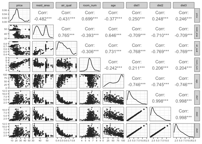
First, a scatter matrix that will give us much relevant information. It has:
- the response variable of our model,
price, plotted against the rest of the variables; - frequency diagrams at the diagonal, so you get a glance of the data distribution;
- scatter plots at the bottom to see how variables are related to each other, and
- Pearson’s correlation coefficients at the upper section. Check this Wikipedia article if you are not familiar with it.
my_ggpairs <- function(data, num_vars){
  num_vars <- enquo(num_vars)

  data %>%
    filter(across(everything(), ~!is.na(.x))) %>%
    select(!!num_vars) %>%
    ggpairs(lower = list(continuous = wrap("points", color = "#333333", shape = 1, size = .5))) +
    theme(axis.text = element_text(size = 6),
          panel.grid.major.x = element_blank(),
          strip.text.x = element_text(size = rel(.8)),
          strip.text.y = element_text(size = rel(.6)))
}

house %>% my_ggpairs(price:dist3)
house %>% my_ggpairs(c(price, dist4:parks, -airport, -waterbody, -bus_ter))
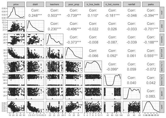
Maybe, you have noticed that:
- Variables like
room_num,teachers, andpoor_prop, are linearly related to thepricefeature. It can be glimpsed in the scatter plots, and they present a correlation coefficient between -1 and -0.5 and between 0.5 and 1, meaning that those relationships are considered strong (it is a convention). - All
distvariables are highly correlated with each other. This high level of correlation between explanatory variables is known as multicollinearity. We are interested in linear relationships between predictors and the response variable. Nevertheless, when predictors are correlated to each other, they do not give us relevant information. Commonly, you only take one of the variables that present multicolinearity and leave the others out of the model. n_hot_roomstakes a range of discrete values, although it is a numeric variable. It has to do with the data collection process or could be a posterior aggregation. By now, let’s consider it as numeric.- Our response variable,
price, seems to have a distribution close to the normal distribution. - Other distributions are skewed to the left or the right. As a follow-up to this exercise, we could try to transform these variables with the appropriate transformation for each case to verify if they would improve our model performance.
Now, It’s the turn of the categorical variables.
house %>% transmute(across(all_of(cat_vars), as.factor)) %>% summary() %>% my_kable(full_width = F)
| airport | waterbody | bus_ter | Sold | |
|---|---|---|---|---|
| NO :230 | Lake : 97 | YES:506 | 0:276 | |
| YES:276 | Lake and River: 71 | 1:230 | ||
| None :155 | ||||
| River :183 |
- There are no missing values among categorical variables; they would have shown up if there were.
bus_terhas onlyYESvalues.
We can consider that bus_ter is a variable of zero variance. It is an uninformative predictor that could ruin the model you want to fit your data.
Another common issue in data sets is near-zero variance predictors. It happens all the time. You’ll find variables that are almost a constant in your data set. It often happens, for example, with categorical data transformed into dummy variables. In general, the preferred approach is keeping all the information possible.
Let’s check how we are with the data regarding this matter.
map_dfr(
  house %>% select(all_of(num_vars)),
  ~ list(Sd = sd(.x, na.rm = TRUE), Var = var(.x, na.rm = TRUE))
) %>%
  add_column(Variable = num_vars, .before = 1) %>%
  my_kable(full_width = FALSE)
| Variable | Sd | Var |
|---|---|---|
| price | 9.1822 | 84.3124 |
| resid_area | 6.8604 | 47.0644 |
| air_qual | 0.1159 | 0.0134 |
| room_num | 0.7026 | 0.4937 |
| age | 28.1489 | 792.3584 |
| dist1 | 2.1085 | 4.4459 |
| dist2 | 2.1086 | 4.4461 |
| dist3 | 2.1198 | 4.4935 |
| dist4 | 2.0992 | 4.4067 |
| teachers | 2.1649 | 4.6870 |
| poor_prop | 7.1411 | 50.9948 |
| n_hos_beds | 1.4767 | 2.1806 |
| n_hot_rooms | 51.5786 | 2660.3489 |
| rainfall | 12.5137 | 156.5926 |
| parks | 0.0106 | 0.0001 |
We can now see that air_qual has a very low standard deviation and variance, and parks shows near-zero variance.
Both quantitative features ranges are very narrow, as we saw at the beginning of this section. In advance, we’d think that those near-zero variances mean that the variables do not hold decisive information. However, we have to be sure before removing any information at all of the data set.
One way to double-check it is using the caret package. It has the nearZeroVar() function to analyze this.
nearZeroVar(house, saveMetrics = TRUE) %>% my_kable(full_width = FALSE)
| freqRatio | percentUnique | zeroVar | nzv | |
|---|---|---|---|---|
| price | 2.000 | 45.0593 | FALSE | FALSE |
| resid_area | 4.400 | 15.0198 | FALSE | FALSE |
| air_qual | 1.278 | 16.0079 | FALSE | FALSE |
| room_num | 1.000 | 88.1423 | FALSE | FALSE |
| age | 10.750 | 70.3557 | FALSE | FALSE |
| dist1 | 1.000 | 66.9960 | FALSE | FALSE |
| dist2 | 1.200 | 69.9605 | FALSE | FALSE |
| dist3 | 1.000 | 66.9960 | FALSE | FALSE |
| dist4 | 1.400 | 69.7628 | FALSE | FALSE |
| teachers | 4.118 | 9.0909 | FALSE | FALSE |
| poor_prop | 1.000 | 89.9209 | FALSE | FALSE |
| airport | 1.200 | 0.3953 | FALSE | FALSE |
| n_hos_beds | 1.000 | 89.7233 | FALSE | FALSE |
| n_hot_rooms | 1.000 | 76.4822 | FALSE | FALSE |
| waterbody | 1.181 | 0.7905 | FALSE | FALSE |
| rainfall | 1.053 | 8.3004 | FALSE | FALSE |
| bus_ter | 0.000 | 0.1976 | TRUE | TRUE |
| parks | 1.000 | 94.4664 | FALSE | FALSE |
| Sold | 1.200 | 0.3953 | FALSE | FALSE |
So, we’ll only consider the variable bus_ter as a zero variance feature.
Missing values and outliers
As we saw before, there are missing values only at n_hos_beds. You may get to understand better why these are missing by looking at the corresponding rows.
house %>% filter(is.na(n_hos_beds)) %>%
  my_kable() %>%
  scroll_box(width = "100%")
| price | resid_area | air_qual | room_num | age | dist1 | dist2 | dist3 | dist4 | teachers | poor_prop | airport | n_hos_beds | n_hot_rooms | waterbody | rainfall | bus_ter | parks | Sold |
|---|---|---|---|---|---|---|---|---|---|---|---|---|---|---|---|---|---|---|
| 19.7 | 39.69 | 0.585 | 5.390 | 72.9 | 2.86 | 2.61 | 2.98 | 2.74 | 20.8 | 21.14 | NO | 121.58 | River | 44 | YES | 0.0610 | 0 | |
| 22.6 | 48.10 | 0.770 | 6.112 | 81.3 | 2.78 | 2.38 | 2.56 | 2.31 | 19.8 | 12.67 | NO | 141.81 | Lake | 26 | YES | 0.0742 | 0 | |
| 25.0 | 40.59 | 0.489 | 6.182 | 42.4 | 4.15 | 3.81 | 3.96 | 3.87 | 21.4 | 9.47 | NO | 12.20 | Lake | 30 | YES | 0.0479 | 0 | |
| 18.8 | 40.01 | 0.547 | 5.913 | 92.9 | 2.55 | 2.23 | 2.56 | 2.07 | 22.2 | 16.21 | YES | 151.50 | River | 35 | YES | 0.0576 | 0 | |
| 19.7 | 35.64 | 0.439 | 5.963 | 45.7 | 7.08 | 6.55 | 7.00 | 6.63 | 23.2 | 13.45 | YES | 111.58 | River | 21 | YES | 0.0404 | 1 | |
| 33.8 | 33.97 | 0.647 | 7.203 | 81.8 | 2.12 | 1.95 | 2.37 | 2.01 | 27.0 | 9.59 | YES | 112.70 | Lake | 21 | YES | 0.0680 | 1 | |
| 7.5 | 48.10 | 0.679 | 6.782 | 90.8 | 1.90 | 1.54 | 2.04 | 1.80 | 19.8 | 25.79 | YES | 10.06 | River | 35 | YES | 0.0646 | 1 | |
| 8.3 | 48.10 | 0.693 | 5.349 | 96.0 | 1.75 | 1.38 | 1.88 | 1.80 | 19.8 | 19.77 | YES | 150.66 | River | 40 | YES | 0.0677 | 1 |
No other value in the rest of the features raises suspicion.
Let’s replace the missing values in the n_hos_beds with the median of the variable. It is just one valid approach, which I consider preferable because you do not lose information. Besides, there are only a few missing values.
house_complete <- house %>%
  mutate(n_hos_beds = case_when(
    is.na(n_hos_beds) ~ median(n_hos_beds, na.rm = TRUE),
    TRUE ~ n_hos_beds
  ))
Outliers are a pain in the neck when you want to fit a particular type of model. Linear Regression is one of them.
An excellent tool to detect outliers are box plots.
house_complete %>%
  select(all_of(num_vars)) %>%
  pivot_longer(names(.), names_to = "variable", values_to = "valor") %>% ggplot(aes(variable, valor)) +
  geom_boxplot(fill = "grey89", outlier.shape = 1) +
  facet_wrap(variable ~ ., scales = "free") +
  labs(x = NULL) +
  theme(axis.text.x = element_blank(),
        axis.text.y = element_text(size = 8))
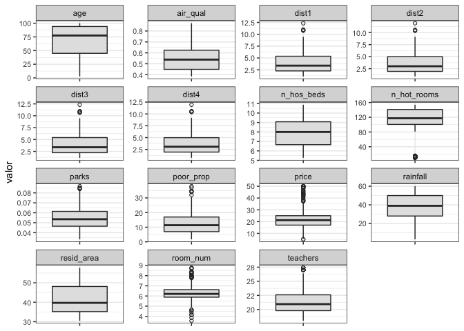
Many variables present values out of the box plot whiskers. In most cases, there is no clear boundary to determine which points are outliers. They form a continuum.
There is just one case where we can be sure that the values are outliers in the n_hot_rooms variable. A set of observations are far from the rest.
Those cases are 125. They are many. It could be due to two reasons: they are measurement errors, or those are cities with a meager amount of hotels, as being non-touristic places.
Let’s show them with the other variables with values outside of the box plot whiskers.
house_complete %>%
  filter(n_hot_rooms < 40) %>%
  head() %>%
  my_kable() %>%
  scroll_box(width = "100%")
| price | resid_area | air_qual | room_num | age | dist1 | dist2 | dist3 | dist4 | teachers | poor_prop | airport | n_hos_beds | n_hot_rooms | waterbody | rainfall | bus_ter | parks | Sold |
|---|---|---|---|---|---|---|---|---|---|---|---|---|---|---|---|---|---|---|
| 5 | 48.10 | 0.693 | 5.453 | 100.0 | 1.57 | 1.26 | 1.79 | 1.34 | 19.8 | 30.59 | NO | 9.30 | 13.04 | Lake | 26 | YES | 0.0653 | 0 |
| 12 | 48.10 | 0.614 | 5.304 | 97.3 | 2.28 | 1.99 | 2.41 | 1.73 | 19.8 | 24.91 | NO | 9.34 | 15.10 | Lake | 39 | YES | 0.0619 | 0 |
| 14 | 51.89 | 0.624 | 6.174 | 93.6 | 1.86 | 1.54 | 1.87 | 1.18 | 18.8 | 24.16 | NO | 5.68 | 10.11 | Lake | 28 | YES | 0.0570 | 0 |
| 18 | 51.89 | 0.624 | 6.431 | 98.8 | 1.96 | 1.61 | 1.92 | 1.77 | 18.8 | 15.39 | NO | 8.16 | 14.14 | None | 41 | YES | 0.0564 | 0 |
| 19 | 35.19 | 0.515 | 5.985 | 45.4 | 4.89 | 4.64 | 5.05 | 4.67 | 19.8 | 9.74 | NO | 6.38 | 11.15 | Lake | 28 | YES | 0.0477 | 0 |
| 20 | 35.96 | 0.499 | 5.841 | 61.4 | 3.39 | 3.28 | 3.62 | 3.22 | 20.8 | 11.41 | NO | 7.50 | 15.16 | None | 39 | YES | 0.0454 | 0 |
The rest of the features show values within the inner quantiles.
There are two things that we can do. Drop those observations or replace the outlier values with other (e.g., the mean, a.k.a. the expected value or the minimum).
In another context, we may have the chance to get more information about the data set we are dealing with, but we cannot go any further in this case.
I’ll consider these outliers as errors in the data collection process and replace them with a central value like the median.
In the next code snippet I save my cleaned data in the new house_prepared variable.
house_prepared <- house_complete %>%
  mutate(n_hot_rooms = case_when(
    n_hot_rooms < 40 ~ median(n_hot_rooms, na.rm = T),
    TRUE             ~ n_hot_rooms
  ))
Another approach with outliers and normally distributed data is the z-score. It is a useful technique if your variable is normally distributed.
The process consists in:
- Standardizing the variable by subtracting the mean and dividing each observation with the variable’s standard deviation.
- Leaving out those values observed at more than three standard deviations of the mean (absolute value of z greater than 3), which will be zero after the standardization.
It is the case of room_num. Now, I’ll show you the observations that are outside these boundaries.
house_prepared %>%
  select(room_num) %>%
  mutate(room_num_z = (room_num - mean(room_num)) / sd(room_num)) %>%
  filter(abs(room_num_z) > 3) %>%
  arrange(room_num_z) %>%
  my_kable(full_width = FALSE)
| room_num | room_num_z |
|---|---|
| 3.561 | -3.876 |
| 3.863 | -3.447 |
| 4.138 | -3.055 |
| 4.138 | -3.055 |
| 8.398 | 3.008 |
| 8.704 | 3.443 |
| 8.725 | 3.473 |
| 8.780 | 3.551 |
Again, it’s a matter of choosing between deleting or replacing those values. I’ll replace them with the maximum to preserve some of the variance.
house_prepared <- house_prepared %>%
  mutate(room_num = case_when(
    room_num <= 4.138 | room_num >= 8.398 ~ median(room_num, na.rm = TRUE),
    TRUE ~ room_num ))
Create a test set
For those who may ask, the usual procedure at this point in a Machine Learning project is, before doing anything else, to create the test set. Set aside a part of the data and not touch it until you get a definitive fine-tuned model.
In this case, I’ll focus more on the inferential side of the Linear Regression than on the model’s predictive power. So I won’t split the data into training and testing sets. I’ll use it as is.
Linear Regression model
Simple Linear Regression
Let’s start simple. I’ll fit a model with price explained by teachers and another defined by poor_prop.
In R, we use the formula syntax. It’s a very intuitive way of writing your model. You place your target variable on the left-hand side of the formula and the features you want on the right-hand side and split them with a tilde symbol (~).
The coefficients estimated for the first model are these.
lm.simple_1 <- lm(price ~ teachers, data = house_prepared)
lm.simple_1$coefficients %>% my_kable(full_width = FALSE)
| x | |
|---|---|
| (Intercept) | -23.676 |
| teachers | 2.145 |
So, we can represent the model with the following expression.
\[\overline{y} = -23.676 +2.145\cdot teachers\]And the coefficients for the second one.
lm.simple_2 <- lm(price ~ poor_prop, data = house_prepared)
lm.simple_2$coefficients %>% my_kable(full_width = FALSE)
| x | |
|---|---|
| (Intercept) | 34.5820 |
| poor_prop | -0.9526 |
Moreover, the model would be the next.
\[\overline{y} = 34.582 -0.953\cdot poor\_prop\]You get how this works.
Differences between models
To get a better understanding of the results, let’s use the summary() function.
summary(lm.simple_1)
##
## Call:
## lm(formula = price ~ teachers, data = house_prepared)
##
## Residuals:
##     Min      1Q  Median      3Q     Max
## -18.783  -4.774  -0.633   3.147  31.212
##
## Coefficients:
##             Estimate Std. Error t value Pr(>|t|)
## (Intercept)  -23.676      3.529   -6.71  5.3e-11 ***
## teachers       2.145      0.163   13.16  < 2e-16 ***
## ---
## Signif. codes:  0 '***' 0.001 '**' 0.01 '*' 0.05 '.' 0.1 ' ' 1
##
## Residual standard error: 7.93 on 504 degrees of freedom
## Multiple R-squared:  0.256,	Adjusted R-squared:  0.254
## F-statistic:  173 on 1 and 504 DF,  p-value: <2e-16
summary(lm.simple_2)
##
## Call:
## lm(formula = price ~ poor_prop, data = house_prepared)
##
## Residuals:
##    Min     1Q Median     3Q    Max
##  -9.95  -4.00  -1.33   2.09  24.50
##
## Coefficients:
##             Estimate Std. Error t value Pr(>|t|)
## (Intercept)  34.5820     0.5588    61.9   <2e-16 ***
## poor_prop    -0.9526     0.0385   -24.8   <2e-16 ***
## ---
## Signif. codes:  0 '***' 0.001 '**' 0.01 '*' 0.05 '.' 0.1 ' ' 1
##
## Residual standard error: 6.17 on 504 degrees of freedom
## Multiple R-squared:  0.549,	Adjusted R-squared:  0.548
## F-statistic:  613 on 1 and 504 DF,  p-value: <2e-16
In the model with teachers as an independent variable:
- The slope of the regression line ($\beta_1$ estimate) tells us that the relation with
priceis positive (as we saw in the correlation plot). It means that when the proportion of teachers in the city rises, so does the house’s price. - It’s coefficient of determination $R^2$, lower than the other one, tells us that this model explains less of the variability embedded in the data.
In the model with poor_prop as the independent variable:
- The negative sign of the coefficient indicates a negative relationship between those variables. It seems that, as the proportion of poor people in the city grows, the price of the household descent.
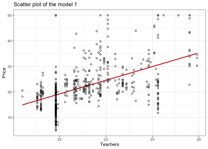
Scatter plot of each model
title <- "Scatter plot of the model 1"
house_prepared %>%
  ggplot(aes(teachers, price)) +
  geom_smooth(method = "lm", color = "firebrick3", fill = NA) +
  geom_point(shape = 1) +
  labs(title = title, x = "Teachers", y = "Price")
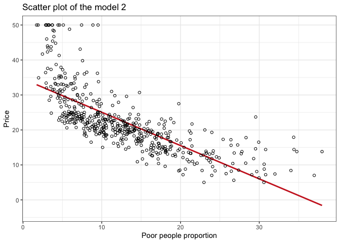
title <- "Scatter plot of the model 2"
house_prepared %>%
  ggplot(aes(poor_prop, price)) +
  geom_smooth(method = "lm", color = "firebrick3", fill = NA) +
  geom_point(shape = 1) +
  labs(title = title, x = "Poor people proportion", y = "Price")
In the scatter plot of model 1:
- We can see a trend between the data points, although the slope is mild.
- The data points show up with a large dispersion around the regression line.
- It stands out some vertical lines across the data points. It’s quite clear near the
xvalue of 20. - There’s another horizontal pattern of this type at the
yaxis value of 50.
In the context of a Machine learning project, you shouldn’t leave those details behind. It is something that I would check with the people responsible for the data collection process.
In the scatter plot of model 2:
- You’ll detect a more pronounced slope of the regression line.
- Data points are closer to the regression line.
- Once again, the pattern over
price = 50shows up. It could mean that the data was capped for this value.
Multiple Linear Regression (quantitative regressors)
lm.multiple_quantitative <- lm(
  price ~ age + teachers + poor_prop, data = house_prepared
)
Effect of each regressor and interpretation
lm.multiple_quantitative %>% summary() %>% coefficients() %>% my_kable(full_width = T)
| Estimate | Std. Error | t value | Pr(>|t|) | |
|---|---|---|---|---|
| (Intercept) | 6.6416 | 2.9960 | 2.217 | 0.0271 |
| age | 0.0400 | 0.0113 | 3.545 | 0.0004 |
| teachers | 1.1489 | 0.1261 | 9.109 | 0.0000 |
| poor_prop | -0.9172 | 0.0462 | -19.837 | 0.0000 |
- The parameter of
ageis very close to zero. It indicates that this variable has a small weight when determining the price of a house. - On
teachersandpoor_prop, you should note that they have more weighty parameters, although they are lower than the previous section’s simple linear regression models. - The observed t and the p-value given for each descriptor variable determines the null hypothesis that the variable’s coefficient is equal to zero.
- For this model, all p-values obtained are lower than the level of significance, and t statistics are higher as the variable coefficient increases. It indicates that the variables are relevant to the model.
Evaluation of the goodness of adjustment through the adjusted coefficient of determination
The adjusted coefficient of determination is another way to evaluate multiple linear regression models. You use it to soften the naturally occurring increase in the coefficient of determination $R^2$ as you add variables to the model.
You get it from the following expression.
\[R^2_a = 1 - (1 - R^2)\frac{n-1}{n-p-1}\]Where,
- $R^2_a$ is the adjusted $R^2$ or the adjusted coefficient of determination,
- $R^2$ is the coefficient of determination,
- $n$ is the number of observations in your data set, and
- $p$ is the number of features in your model
You get it from the fitted model object like this.
summary(lm.multiple_quantitative)$r.squared
## [1] 0.6191
summary(lm.multiple_quantitative)$adj.r.squared
## [1] 0.6168
Concerning the standard $R^2$, the adjusted coefficient of determination is practically the same. We’ll get the most of this metric afterward.
Extension of the model with the variables room_num, n_hos_beds and n_hot_rooms
Let’s compare the previous model with the following one.
lm.multiple_quantitative_extended <- lm(
  price ~ age + teachers + poor_prop + room_num + n_hos_beds + n_hot_rooms,
  data = house_prepared
)
So now, we see the statistical summary of the model.
summary(lm.multiple_quantitative_extended)
##
## Call:
## lm(formula = price ~ age + teachers + poor_prop + room_num +
##     n_hos_beds + n_hot_rooms, data = house_prepared)
##
## Residuals:
##     Min      1Q  Median      3Q     Max
## -11.977  -3.044  -0.679   2.079  28.365
##
## Coefficients:
##              Estimate Std. Error t value Pr(>|t|)
## (Intercept) -25.43960    4.69790   -5.42  9.5e-08 ***
## age           0.01841    0.01045    1.76   0.0786 .
## teachers      0.97615    0.11610    8.41  4.4e-16 ***
## poor_prop    -0.61365    0.05111  -12.01  < 2e-16 ***
## room_num      4.81766    0.47401   10.16  < 2e-16 ***
## n_hos_beds    0.43317    0.15728    2.75   0.0061 **
## n_hot_rooms  -0.00204    0.01485   -0.14   0.8909
## ---
## Signif. codes:  0 '***' 0.001 '**' 0.01 '*' 0.05 '.' 0.1 ' ' 1
##
## Residual standard error: 5.16 on 499 degrees of freedom
## Multiple R-squared:  0.688,	Adjusted R-squared:  0.685
## F-statistic:  184 on 6 and 499 DF,  p-value: <2e-16
- The t statistic and their associated p-values obtained for
ageandn_hot_roomstell us that these variables are not significant for the model.
However, one thing is that variables are not significant, and the other is that the model is not significant.
In the same inference approach of the modeling process, we use the F-statistic to check if a model significantly explains the response variable Y or not. If we get an F close to one, it means that the model is not significant. But here, we got an F way higher than one and a small p. So, we can consider that our variables are significantly linearly correlated with our response variable.
As we introduced more explanatory variables than the previous model, it is of interest to use $R_a^2$ to compare them.
summary(lm.multiple_quantitative)$adj.r.squared
## [1] 0.6168
summary(lm.multiple_quantitative_extended)$adj.r.squared
## [1] 0.6845
In this case, we see an increase of about 6% in the $R^2$ of the model.
Multiple linear regression models (quantitative and qualitative regressors)
We want to know what happens if we extend the previous model with the airport variable.
lm.multiple_quanti_quali <- lm(
  price ~
    age + teachers + poor_prop + room_num + n_hos_beds + n_hot_rooms + airport,
  data = house_prepared
)
Is the new model significantly better?
summary(lm.multiple_quantitative_extended)$adj.r.squared
## [1] 0.6845
summary(lm.multiple_quanti_quali)$adj.r.squared
## [1] 0.6882
In this case, the improvement obtained, comparing the adjusted $R^2$, is very small.
Prediction of the price of housing
Now, let’s imagine that we want to predict a new house’s price with the following characteristics.
age = 70, teachers = 15, poor_prop = 15, room_num = 8, n_hos_beds = 8, n_hot_rooms = 100
I’ll use the model fitted with quantitative and qualitative variables to perform the prediction. So far, it’s the best one.
new_house <- tibble(
  age = 70,
  teachers = 15,
  poor_prop = 15,
  room_num = 8,
  n_hos_beds = 8,
  n_hot_rooms = 100
)

predict(
  lm.multiple_quantitative_extended,
  new_house,
  interval = "confidence"
) %>%
  data.frame() %>%
  my_kable(full_width = FALSE)
| fit | lwr | upr |
|---|---|---|
| 23.09 | 20.52 | 25.66 |
The model predicts a price in the range $(19,99, 25,20)$ with 95% confidence.
Visual verification of modeling assumptions
I represent the residues against the values estimated by the model in a dispersion diagram.
y_pred <- lm.multiple_quanti_quali$fitted.values
residuals <- summary(lm.multiple_quanti_quali)$residuals

residuals_df <- tibble(y_pred, residuals)

title <- "Residuals vs. Fitted"
residuals_df %>%
  ggplot(aes(y_pred, residuals)) +
  geom_smooth(color = "firebrick3", method = "lm", se = F) +
  geom_point(shape = 1, color = "#333333") +
  labs(title = title, x = "Fitted Values", y = "Residuals")
## `geom_smooth()` using formula 'y ~ x'
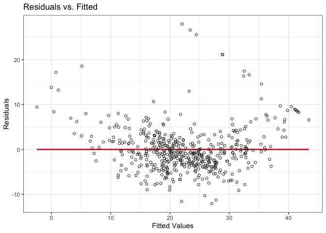
The errors present homoscedasticity; that is, they are evenly distributed around the regression line for residuals, without forming any particular structure.
I check that the mean residue is zero and perform a histogram and hypothesis contrast to test the alternative hypothesis that the residues follow a normal distribution.
residuals_df %>%
  ggplot(aes(residuals)) +
  geom_histogram(bins = 30, fill = "#333333", colour = "white") +
  labs(title = "Residuals distribution", x = "Residuals",  y = "Count")
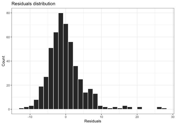
They present a mean of almost 0, and I can accept the hypothesis that the residues follow a normal distribution according to the histogram and the p-value obtained in the normality test.
We can also catch outliers in the dependent variable where the residuals are too far from the line, using the z-score criterion.
residuals_outliers <- residuals_df %>%
  rownames_to_column() %>%
  mutate(residuals_z = (residuals - mean(residuals)) / sd(residuals)) %>%
  filter(abs(residuals_z) > 3) %>%
  pull(rowname)

house_prepared %>% filter(row_number() %in% residuals_outliers) %>% my_kable() %>% scroll_box(width = "100%")
| price | resid_area | air_qual | room_num | age | dist1 | dist2 | dist3 | dist4 | teachers | poor_prop | airport | n_hos_beds | n_hot_rooms | waterbody | rainfall | bus_ter | parks | Sold |
|---|---|---|---|---|---|---|---|---|---|---|---|---|---|---|---|---|---|---|
| 50.0 | 48.10 | 0.631 | 4.970 | 100.0 | 1.47 | 1.11 | 1.52 | 1.23 | 19.8 | 3.26 | NO | 9.700 | 117.3 | River | 41 | YES | 0.0624 | 0 |
| 17.9 | 48.10 | 0.597 | 4.628 | 100.0 | 1.77 | 1.54 | 1.78 | 1.13 | 19.8 | 34.37 | NO | 8.358 | 151.4 | None | 40 | YES | 0.0587 | 0 |
| 50.0 | 36.20 | 0.504 | 6.208 | 83.0 | 3.13 | 2.61 | 2.95 | 2.88 | 22.6 | 4.63 | NO | 7.500 | 117.3 | River | 20 | YES | 0.0570 | 0 |
| 50.0 | 33.97 | 0.647 | 6.208 | 86.9 | 2.09 | 1.53 | 1.83 | 1.76 | 27.0 | 5.12 | NO | 8.600 | 117.3 | River | 54 | YES | 0.0552 | 0 |
| 50.0 | 48.10 | 0.631 | 6.683 | 96.8 | 1.55 | 1.28 | 1.65 | 0.94 | 19.8 | 3.73 | NO | 6.700 | 117.3 | River | 58 | YES | 0.0675 | 0 |
| 50.0 | 48.10 | 0.631 | 7.016 | 97.5 | 1.40 | 0.92 | 1.20 | 1.28 | 19.8 | 2.96 | NO | 10.100 | 117.3 | None | 46 | YES | 0.0592 | 0 |
| 50.0 | 48.10 | 0.631 | 6.216 | 100.0 | 1.38 | 0.95 | 1.36 | 0.99 | 19.8 | 9.53 | NO | 9.800 | 117.3 | None | 25 | YES | 0.0609 | 0 |
| 50.0 | 48.10 | 0.668 | 5.875 | 89.6 | 1.13 | 1.01 | 1.25 | 1.12 | 19.8 | 8.88 | NO | 10.800 | 117.3 | None | 57 | YES | 0.0645 | 0 |
| 23.7 | 40.59 | 0.489 | 5.412 | 9.8 | 3.68 | 3.48 | 3.67 | 3.53 | 21.4 | 29.55 | YES | 5.674 | 111.9 | None | 21 | YES | 0.0561 | 0 |
| 48.8 | 33.97 | 0.647 | 6.208 | 91.5 | 2.55 | 2.04 | 2.39 | 2.17 | 27.0 | 5.91 | YES | 10.076 | 153.9 | River | 24 | YES | 0.0551 | 0 |
We see that practically all cases with price = 50 appear as atypical cases. Other outliers come out among the variables where we couldn’t establish a clear boundary for atypical cases, e.g., for teachers > 27 and poor_prop > 29 (as we saw here).
It will be interesting to see what happens if we adjust the model again, leaving out the outliers detected by analyzing residuals. How do you think that this will affect the model’s performance?
lm(
  price ~ age + teachers + poor_prop + room_num + n_hos_beds + n_hot_rooms,
  data = house_prepared %>% filter(!row_number() %in% residuals_outliers)
) %>%
  summary() %>% .$r.squared
## [1] 0.7768
The $R^2$ of the model improves by almost 10 points regarding the model that includes the outliers!
This phenomenon is known as garbage-in garbage-out in the Machine Learning field. If you feed your model with poor quality data, you’ll get a low-quality model. The best thing you can do if you want to use your model for prediction is retraining it without these noisy observations.
Takeaways
This is what we have learned in this blog post:
- Linear Regression is relatively simple, and so, it is more explainable than other models.
- Be aware of the outliers. Give the data processing step the care that it deserves. Recheck them when you go through the validation of the model’s assumptions.
- Check the model assumptions (independent variable or residuals normally distributed and homoscedasticity) to ensure that what you are doing is right.
- Test different variable combinations to see how you can improve your model’s performance.
That’s it for this post. I hope you have enjoyed it. If you have any comments or suggestions, do not hesitate to contact me!