
Text Processing With Python. First Steps.
Published:
In this post, we will explore text analysis techniques with Python, just scratching the surface of the fascinating field of Natural Language Processing (NLP).

Two years ago, I scraped this Q&A forum about housing in Spain, powered by the housing renting and selling portal enalquiler.com.
The forum was shut down at some point, and it doesn’t admit any new users or questions, but it is opened to the public to allow consulting the Q&A that took place the time the forum was active.
Today I want to scratch the NLP’s surface and see what knowledge we can obtain using a few simple text processing techniques.
Let’s prepare the working environment.
import matplotlib.pyplot as plt
import matplotlib as mpl
import pandas as pd
import numpy as np
import unidecode
import stanza
import spacy
import nltk
import re

from sklearn.feature_extraction.text import TfidfVectorizer
from nltk.tokenize import word_tokenize
from nltk.corpus import stopwords
from collections import Counter
I am also customizing some matplotlib parameters to get nice plots.
plt.style.use('ggplot')

plt.rcParams["grid.alpha"] = 0.9
plt.rcParams["axes.facecolor"] = "#f0f0f0"
plt.rcParams["figure.facecolor"] = "#f0f0f0"
plt.rcParams["figure.figsize"] = (6.4*1.2, 4.8*1.2)
The data
When scraping the data from the forum, I went through each question’s link and got the following information:
id: a unique identifier for each question.user_name: the name of the user making the question.user_category: whether they are a tenant, a landlord, a professional, or a deleted user.quesion_category: the category of the question.question_title: the title of the question.question_body: the question itself.estimated_date: the date that the user formulated the question.url: the URL of the question or answer.
The data I scraped from the web is far more complex. Questions have answers, and users voted them as useful. However, for a matter of simplicity, I’ll stick to questions in this blog post.
I did some data preparation steps previously. If you are curious about what I did, check out this notebook.
Now, let’s get down to business!
First, we load the data set.
questions = pd.read_csv("../data/enalquiler/clean/questions.csv")
questions.shape
(84642, 8)
A considerable amount of questions! Let’s change the date attribute estimated_date to date type and get some information about our data set.
questions.estimated_date = pd.to_datetime(questions.estimated_date)

questions.info(show_counts=True)
<class 'pandas.core.frame.DataFrame'>
RangeIndex: 84642 entries, 0 to 84641
Data columns (total 8 columns):
 #   Column             Non-Null Count  Dtype
---  ------             --------------  -----
 0   id                 84638 non-null  float64
 1   user               82841 non-null  object
 2   user_category      84635 non-null  object
 3   question_category  84603 non-null  object
 4   question_title     84626 non-null  object
 5   question_body      84603 non-null  object
 6   url                84634 non-null  object
 7   estimated_date     84631 non-null  datetime64[ns]
dtypes: datetime64[ns](1), float64(1), object(6)
memory usage: 5.2+ MB
This is how the full data set looks like.
questions.head()
| id | user | user_category | question_category | question_title | question_body | url | estimated_date | |
|---|---|---|---|---|---|---|---|---|
| 0 | 1.405004e+14 | David | inquilino/a | Desahucios | Me reclaman los meses inpagados de mi desaucio | Buenas noches, hace 3 años a día de hoy tuve u... | https://www.enalquiler.com/comunidad-alquiler/... | 2019-01-01 |
| 1 | 1.405004e+14 | keifarem | inquilino/a | Reparaciones | GASTOS DE MANTENIMENTO I RESCATE DEL ASCENSOR | Buenos dias , Hemos alquilado una vivienda qu... | https://www.enalquiler.com/comunidad-alquiler/... | 2019-01-01 |
| 2 | 1.405004e+14 | ana1 | casero/a | Legislación alquiler | FINALIZACION CONTRATO DE ALQUILER | Buenos días Yo tenía firmado un contrato de ... | https://www.enalquiler.com/comunidad-alquiler/... | 2019-01-01 |
| 3 | 1.405004e+14 | Nieves Martin Perez | casero/a | Caseros | AGUJEROS POR USO DE TACOS EN LAS PAREDES | Buenos tardes, Recientemente mi inquilino me a... | https://www.enalquiler.com/comunidad-alquiler/... | 2019-01-01 |
| 4 | 1.405004e+14 | Juan Fco aranda | inquilino/a | Legislación alquiler | Validez del contrato | Hola tengo un contraro del año 2005 y quiero e... | https://www.enalquiler.com/comunidad-alquiler/... | 2019-01-01 |
Quick data exploration
We can start asking questions about our data right away. For instance,
- What type of user has used the forum more? or
- Which are the top trending topics on the forum? or even,
- How many questions people asked each year?
Let’s use some tables and visualizations to help us answer them.
from collections import OrderedDict

users = OrderedDict(questions.user_category.value_counts().sort_values())
user = list(users.keys())
nposts = list(users.values())

def annotate_barh(ax, size, limit, xytext_big, xytext_small):
    for p in ax.patches:
        if p.get_width() > limit:
            ax.annotate(str(p.get_width()), (p.get_x() + p.get_width(), p.get_y()), size=size,
                        xytext=xytext_big, textcoords='offset points', color="white", fontweight="bold")
        else:
            ax.annotate(str(p.get_width()), (p.get_x() + p.get_width(), p.get_y()),
                        xytext=xytext_small, textcoords='offset points', size=size)


fig, ax = plt.subplots(dpi=80)

ax.barh(user, nposts, color="#00bfff")
annotate_barh(ax, size=12, limit=2.0E+03, xytext_big=(-55, 25), xytext_small=(10, 25))
ax.set(ylabel="User Category", xlabel="Count", title="Count of Questions by User Category")

plt.show()
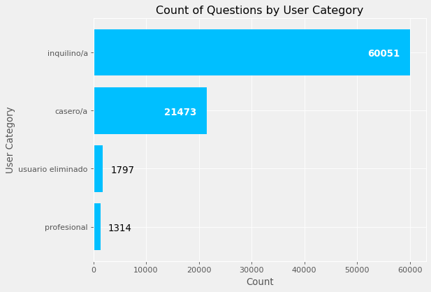
from collections import OrderedDict

user_cat_count = dict(questions.sort_values("id").groupby('id').first()
                      .reset_index().groupby(["user_category"]).size())

user_cat_count_ordered = dict(sorted(user_cat_count.items(), key=lambda item: item[1]))
user_cat = list(user_cat_count_ordered.keys())
nposts = list(user_cat_count_ordered.values())

fig, ax = plt.subplots(dpi=80)

ax.barh(user_cat, nposts, color="#00bfff")

annotate_barh(ax, size=12, limit=2.0E+03, xytext_big=(-55, 25), xytext_small=(10, 25))

ax.set(ylabel="User category", xlabel="Count", title="Count of Questions by User Category")

plt.show()

Most users asking questions were tenants and then landlords.
q_categories = dict()

for key, value in dict(questions.question_category.value_counts()).items():
    if value >= 100:
        q_categories[key] = value

q_categories = dict(sorted(q_categories.items(), key = lambda kv: kv[1]))
q_cat = list(q_categories.keys())
n_posts = list(q_categories.values())

fig, ax = plt.subplots(dpi=80)

ax.barh(q_cat, n_posts, color="#00bfff")

annotate_barh(ax, size=10, limit=5.0E+03, xytext_big=(-35, 2.5), xytext_small=(5, 2.5))

ax.set(title="# of questions by category", xlabel="# of questions", ylabel="Question category")

plt.show()
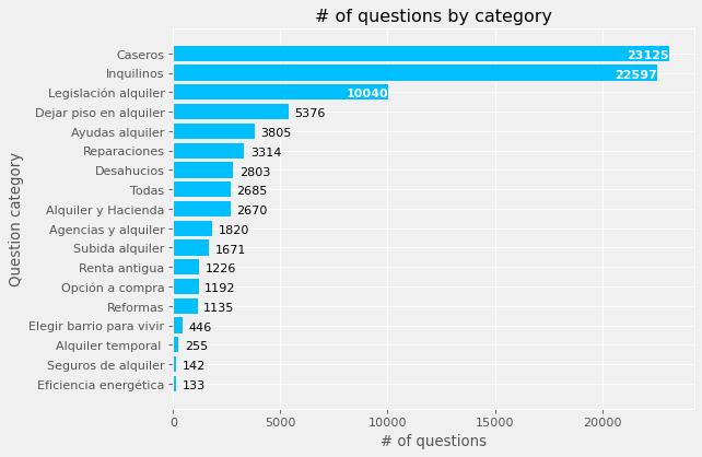
Above are the categories with at least one hundred questions. Notice that “Todas” is not the sum of them altogether, as one might think.
(questions["question_body"].groupby([questions['estimated_date'].dt.year.rename('year')])
                            .agg({'count'})
                            .reset_index(inplace=False))
| year | count | |
|---|---|---|
| 0 | 2008.0 | 2402 |
| 1 | 2009.0 | 11414 |
| 2 | 2010.0 | 13076 |
| 3 | 2011.0 | 12226 |
| 4 | 2012.0 | 12395 |
| 5 | 2013.0 | 7540 |
| 6 | 2014.0 | 5340 |
| 7 | 2015.0 | 5920 |
| 8 | 2016.0 | 4970 |
| 9 | 2017.0 | 3864 |
| 10 | 2018.0 | 3480 |
| 11 | 2019.0 | 1972 |
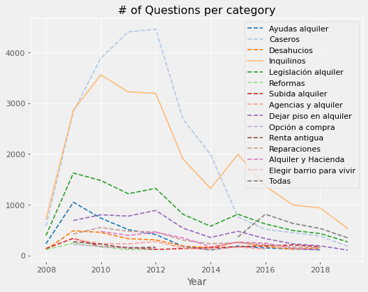
Now, let’s see how the number of questions by category changed over time.
n_q_year_cat = (questions["question_body"]
                .groupby([questions["estimated_date"].dt.year.rename("year"),
                          questions["question_category"]])
                .agg({'count'})
                .reset_index(inplace=False))

n_q_year_cat = n_q_year_cat.loc[n_q_year_cat["count"] > 100,:]

from cycler import cycler

custom_cycler = (cycler(color=plt.cm.get_cmap("tab20").colors[0:16]) +
                cycler(linestyle=["--", "--", "--"] + ["-"] + ["--" for i in range(12)]))

fig, ax = plt.subplots(dpi=80)

ax.set_prop_cycle(custom_cycler)
for cat in pd.unique(n_q_year_cat["question_category"]):
    ax.plot(n_q_year_cat.loc[n_q_year_cat["question_category"] == cat, "year"],
            n_q_year_cat.loc[n_q_year_cat["question_category"] == cat, "count"],
            label=cat)

ax.set(xlabel="Year", title="# of Questions per category")
ax.legend()

plt.show()
The Text Processing Workflow
Let’s say that we are working with the sentence “Text processing isn’t that hard. I bet you 10€ that you can understand it”. I summarize the most common steps when working with text in the following table. Check out this comprehensive blog post if you want a more in-depth explanation.
| Step | Description | Example |
|---|---|---|
| Normalization | Remove special characters, numbers, capital letters, and punctuation | text processing is nt that hard i bet you that you can understand it |
| Removing Stopwords | Remove words that do not give meaning in the context | text processing hard bet understand |
| Tokenization | Splitting text into smaller peaces | <”text”, “processing”, “hard”, “bet”, “understand”> |
| Lemmatization | Reducing words to their root-base form | text processing hard bet understand |
| Stemming | Reducing words to their root-base form but having different variations | text process hard bet understand |
As you can see, stemming is a similar procedure to lemmatization, but the former is based on heuristics, so it tends to produce more errors. This resource is excellent to understand the difference. I’ll stick to lemmatization in this case.
I won’t cover other more advanced topics like POS tagging here, but it deserves to check out to dig deeper in text processing.
I’ll join together question_title and question_body previous to the text processing work, as both comprise relevant information. I’ll override our questions variable with the result and the user category, as they are the only matter of interest from now on.
questions["full_question"] = questions["question_title"] + " " + questions["question_body"]
questions = questions[["user_category", "full_question"]]
Normalization
So, we normalize the text (i.e., remove all numbers, symbols, unnecessary white spaces, coding it to UTF-8 and lower casing the letters). We can do this with a function.
def clean_text(df, text_field, new_text_field_name):
    cleaning_regex = "(@[A-Za-z0-9]+)|([^0-9A-Za-z \t])|(\w+:\/\/\S+)"
    df[new_text_field_name] = (df[text_field].str.lower()
                               .str.normalize('NFKD').str.encode('ascii', errors='ignore').str.decode('utf-8')
                               .apply(lambda t: re.sub(cleaning_regex, "", str(t)))
                               .apply(lambda elem: re.sub(r"\d+", "", elem)))
    return df

questions = clean_text(questions, "full_question", "full_question_clean")
Remove Stop Words
The next thing to do is removing the stop words. Those are words that frequently appear in a text but do not give any insightful meaning. In English, it would be the word the, for example. In Spanish, these are a few of them.
nltk.download("stopwords", quiet=True)
stop_words = stopwords.words("spanish")

stop_words[0:10]
['de', 'la', 'que', 'el', 'en', 'y', 'a', 'los', 'del', 'se']
def remove_stop_words(df, column, stop_words_list):
    try:
        return df[column].apply(lambda x: " ".join([w for w in x.split() if w not in stop_words_list]))
    except:
        return df[column].apply(lambda x: [w for w in x if w not in stop_words_list])

questions["full_question_clean"] = remove_stop_words(questions, "full_question_clean", stop_words)
Tokenization
We have reduced some of the noise present in our data. But we need to go further in this sense.
Tokenization consists of splitting a larger linguistic entity into smaller pieces. If you have a text, sentences are tokens of this text, and words are tokens of the sentences.
Tokenization will give us the possibility to compare questions in terms of concepts. As we have removed some words that won’t mean anything, we might find some others after applying tokenization and counting each word’s occurrences.
questions["question_tokens"] = questions["full_question_clean"].apply(lambda x: word_tokenize(x))
After the transformations, the data looks like this.
questions.head()
| user_category | full_question | full_question_clean | question_tokens | |
|---|---|---|---|---|
| 0 | inquilino/a | Me reclaman los meses inpagados de mi desaucio... | reclaman meses inpagados desaucio buenas noche... | [reclaman, meses, inpagados, desaucio, buenas,... |
| 1 | inquilino/a | GASTOS DE MANTENIMENTO I RESCATE DEL ASCENSOR ... | gastos mantenimento i rescate ascensor buenos ... | [gastos, mantenimento, i, rescate, ascensor, b... |
| 2 | casero/a | FINALIZACION CONTRATO DE ALQUILER Buenos días... | finalizacion contrato alquiler buenos dias ten... | [finalizacion, contrato, alquiler, buenos, dia... |
| 3 | casero/a | AGUJEROS POR USO DE TACOS EN LAS PAREDES Bueno... | agujeros uso tacos paredes buenos tardes recie... | [agujeros, uso, tacos, paredes, buenos, tardes... |
| 4 | inquilino/a | Validez del contrato Hola tengo un contraro de... | validez contrato hola contraro ano quiero empa... | [validez, contrato, hola, contraro, ano, quier... |
With this operation, now we can go through the most common terms that the users included in the questions. Let’s represent the top-10 most used words in a plot.
def plot_topn_word_counts(df, word_column, top_n = 20):
    word_list = [item for sublist in df[word_column] for item in sublist]
    counts = dict(Counter(word_list))
    counts = dict(sorted(counts.items(), reverse=True, key=lambda item: item[1]))

    df = pd.DataFrame({
        "word": list(counts.keys())[0:top_n],
        "count" : list(counts.values())[0:top_n]
    })

    df.sort_values("count",inplace=True)

    plt.rcParams.update({"figure.autolayout": True})

    fig, ax = plt.subplots(dpi= 80)

    ax.barh(df["word"], df["count"], color="#00bfff")

    annotate_barh(ax, size=12, limit=3.5E+04, xytext_big=(-50, 2.5), xytext_small=(5, 2.5))

    ax.set(xlabel="Word count", title="Most Frequent Words")

    plt.show()

plot_topn_word_counts(questions, "question_tokens")
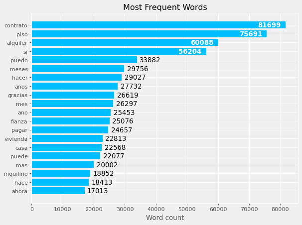
If you know Spanish, you may have noticed some other words that are not so useful. We can remove those to get a better idea of what the users comment on in the forum. I pulled a few more that I found after doing this process iteratively.
more_stop_words = ["si", "meses", "gracias", "hacer", "puedo", "mes", "anos", "ano", "parte", "saber", "él",
                   "casa", "hace", "mas", "puede", "ahora", "dos", "dice", "hola", "q", "muchas", "pago", "ir", "yo",
                   "solo", "asi", "dia", "debo", "quiere", "caso", "quiero", "mas", "dias", "dicho", "buenas", "hacer"]

questions["question_tokens"] = remove_stop_words(questions, "question_tokens", more_stop_words)

plot_topn_word_counts(questions, "question_tokens")
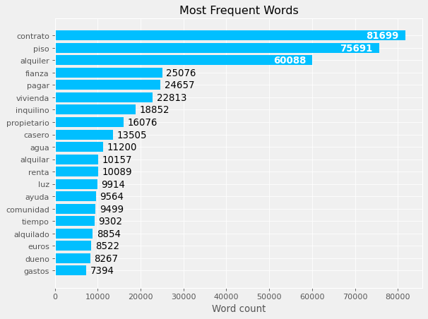
Well! It looks much better now.
In my opinion:
- It is expected to find words like “flat”, “household”, “landlord” or “tenant”.
- Some other words are a clear reference to a specific topic: “deposit”, “water”, “light”, “time”, “community” seems to be the main topics in the forum.
Lemmatization
Lemmatization helps us preserving the meaning of the word while taking it to its root form. It’s a technique based on algorithms. That is why it is preferred over stemming, which relies on heuristics.
sample_list = questions.loc[0, "question_tokens"]

sample = [sample_list[idx] for idx in [0, 1]]

nlp = spacy.load("es_core_news_sm", disable=['parser', 'tagger', 'ner'])
doc = nlp(" ".join(sample))

print(sample)
print([w.lemma_ for w in doc])
['reclaman', 'inpagados']
['reclamar', 'inpagado']
questions["question_lemmas"] = questions["question_tokens"].apply(lambda x: [y.lemma_ for y in nlp(" ".join(x))])
questions
| user_category | full_question | full_question_clean | question_tokens | question_lemmas | |
|---|---|---|---|---|---|
| 0 | inquilino/a | Me reclaman los meses inpagados de mi desaucio... | reclaman meses inpagados desaucio buenas noche... | [reclaman, inpagados, desaucio, noches, hoy, d... | [reclamar, inpagado, desaucio, noches, hoy, de... |
| 1 | inquilino/a | GASTOS DE MANTENIMENTO I RESCATE DEL ASCENSOR ... | gastos mantenimento i rescate ascensor buenos ... | [gastos, mantenimento, i, rescate, ascensor, b... | [gasto, mantenimento, i, rescate, ascensor, bu... |
| 2 | casero/a | FINALIZACION CONTRATO DE ALQUILER Buenos días... | finalizacion contrato alquiler buenos dias ten... | [finalizacion, contrato, alquiler, buenos, ten... | [finalizacion, contrato, alquiler, buen, tenia... |
| 3 | casero/a | AGUJEROS POR USO DE TACOS EN LAS PAREDES Bueno... | agujeros uso tacos paredes buenos tardes recie... | [agujeros, uso, tacos, paredes, buenos, tardes... | [agujero, uso, taco, pared, buen, tarde, recie... |
| 4 | inquilino/a | Validez del contrato Hola tengo un contraro de... | validez contrato hola contraro ano quiero empa... | [validez, contrato, contraro, empadronar, ccun... | [validez, contrato, contraro, empadronar, ccun... |
| ... | ... | ... | ... | ... | ... |
| 84637 | inquilino/a | ¿A quién le reclamo si nadie sabe nada de la R... | reclamo si nadie sabe renta basica emancipacio... | [reclamo, nadie, sabe, renta, basica, emancipa... | [reclamo, nadie, saber, renta, basico, emancip... |
| 84638 | casero/a | Si tengo un piso de proteccion oficial, ¿puedo... | si piso proteccion oficial puedo alquilarlo du... | [piso, proteccion, oficial, alquilarlo, duraci... | [piso, proteccion, oficial, alquilar él, durac... |
| 84639 | inquilino/a | ¿Puedo irme de un piso por mala convivencia y ... | puedo irme piso mala convivencia devuelvan fia... | [irme, piso, mala, convivencia, devuelvan, fia... | [ir yo, piso, malo, convivencia, devuelir, fia... |
| 84640 | inquilino/a | He pedido la ayuda de emancipación, la tenemos... | pedido ayuda emancipacion concedida enero mand... | [pedido, ayuda, emancipacion, concedida, enero... | [pedido, ayuda, emancipacion, concedido, enero... |
| 84641 | casero/a | Si los inquilinos se van antes de finalizar el... | si inquilinos van finalizar contrato entregar ... | [inquilinos, van, finalizar, contrato, entrega... | [inquilino, ir, finalizar, contrato, entregar,... |
84642 rows × 5 columns
TF-IDF
TF-IDF accounts for Term Frequency (multiplied by) Inverse of Document Frequency. You can find a detailed explanation in this fantastic medium post.
In short, this metric gives us what words are unique for a document. It’s a metric of what texts are about.
So, we have to create a separate document for each group of text we want to compare. In our context, a document will be the questions, joined all together by user category. I’ll use the processed text stored in question_lemmas to do it.
inquilinos = questions.loc[questions.user_category == "inquilino/a", "question_lemmas"]
caseros = questions.loc[questions.user_category == "casero/a", "question_lemmas"]
usuarios_eliminados = questions.loc[questions.user_category == "usuario eliminado", "question_lemmas"]
profesionales = questions.loc[questions.user_category == "profesional", "question_lemmas"]
Then, we create each document. I.e., the groups of text that we want to analyze with the TF-IDF technique.
doc_tenants = " ".join([item for sublist in inquilinos.values for item in sublist])
doc_landlords = " ".join([item for sublist in caseros.values for item in sublist])
doc_removed_users = " ".join([item for sublist in usuarios_eliminados.values for item in sublist])
doc_professionals = " ".join([item for sublist in profesionales.values for item in sublist])
I’ll use the TfidfVectorizer() class from Sci-kit Learn, which calculates the TF-IDF score for the words in the different documents in a pipeline. The result is a feature matrix with the actual terms and their scores.
vectorizer = TfidfVectorizer()

vectors = vectorizer.fit_transform([doc_tenants, doc_landlords, doc_removed_users, doc_professionals])

feature_names = vectorizer.get_feature_names()
dense = vectors.todense()
denselist = dense.tolist()

tfidf_matrix = pd.DataFrame(denselist, columns=feature_names)
The higher scores in each matrix row go to the words that are more specific for each document. The resulting matrix looks like this.
tfidf_matrix.head()
| aa | aaaaaa | aabagir | aabierto | aabogado | aabonar | aabril | aabro | aac | aacabo | ... | zurich | zusendenmattheu | zwembadhuurir | zón | án | ás | él | és | ín | ún | |
|---|---|---|---|---|---|---|---|---|---|---|---|---|---|---|---|---|---|---|---|---|---|
| 0 | 0.000326 | 0.000014 | 0.000014 | 0.000000 | 0.000014 | 0.000014 | 0.000014 | 0.000014 | 0.000022 | 0.000000 | ... | 0.000014 | 0.000014 | 0.000014 | 0.000788 | 0.000335 | 0.000014 | 0.231720 | 0.000000 | 0.000022 | 0.000014 |
| 1 | 0.000279 | 0.000000 | 0.000000 | 0.000044 | 0.000000 | 0.000000 | 0.000000 | 0.000000 | 0.000034 | 0.000044 | ... | 0.000000 | 0.000000 | 0.000000 | 0.000530 | 0.000362 | 0.000000 | 0.299099 | 0.000044 | 0.000034 | 0.000000 |
| 2 | 0.000000 | 0.000000 | 0.000000 | 0.000000 | 0.000000 | 0.000000 | 0.000000 | 0.000000 | 0.000000 | 0.000000 | ... | 0.000000 | 0.000000 | 0.000000 | 0.000000 | 0.000303 | 0.000000 | 0.249843 | 0.000000 | 0.000000 | 0.000000 |
| 3 | 0.000559 | 0.000000 | 0.000000 | 0.000000 | 0.000000 | 0.000000 | 0.000000 | 0.000000 | 0.000000 | 0.000000 | ... | 0.000000 | 0.000000 | 0.000000 | 0.001119 | 0.000000 | 0.000000 | 0.271202 | 0.000000 | 0.000000 | 0.000000 |
4 rows × 104596 columns
Finally, we can transpose it to represent TF-IDF and see what we can learn about our data set.
tfidf = tfidf_matrix.T

tfidf.rename(columns={0:"tenant", 1:"landlord", 2:"removed_user", 3:"professional"}, inplace=True)

plt.rcParams.update({"figure.autolayout": True})

fig, axes = plt.subplots(2, 2, facecolor='#f0f0f0')

tfidf_tenants = tfidf.sort_values(["tenant"], ascending=False)[["tenant"]]
tfidf_landlords = tfidf.sort_values(["landlord"], ascending=False)[["landlord"]]
tfidf_removed_user = tfidf.sort_values(["removed_user"], ascending=False)[["removed_user"]]
tfidf_pro = tfidf.sort_values(["professional"], ascending=False)[["professional"]]

ax1 = axes[0, 0]
ax1.barh(tfidf_tenants.index[10::-1], tfidf_tenants.tenant[10::-1], color="#00bfff")
ax1.set(xlabel="TF-IDF", title="Tenants")

ax2 = axes[0, 1]
ax2.barh(tfidf_landlords.index[10::-1], tfidf_landlords.landlord[10::-1], color="#f58f29")
ax2.set(xlabel="TF-IDF", title="Landlords")

ax3 = axes[1, 0]
ax3.barh(tfidf_removed_user.index[10::-1], tfidf_removed_user.removed_user[10::-1], color="#66101f")
ax3.set(xlabel="TF-IDF", title="Removed Users")

ax4 = axes[1, 1]
ax4.barh(tfidf_pro.index[10::-1], tfidf_pro.professional[10::-1], color="#73628a")
ax4.set(xlabel="TF-IDF", title="Professionals")

plt.show()
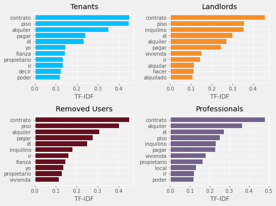
- As expected, the most frequent and particular words of each of the users are “contrato” (contract), “piso” (apartment).
- We should perform more complex analysis to get actual context on what each type of user asked about.
Recap
In this blog post, we have:
- Analized text data visually to get insights
- Performed some text processing operations, like normalization, removing stop words, tokenization, and lemmatization
- Used the TDF-IDF vectorizer technique to get the words that are more characteristic for each document when compared.
That’s it for this post. Let me know if you liked it or if you have any questions or suggestions!